|

|
|
|
Background The CMB (cosmic microwave background)
consists of light emitted a mere 380 thousand years after the
big bang when the universe was less than 0.002% of its current age. This light comes from what is known as the surface
of last scattering -- the time when the universe cooled enough to allow
protons to capture electrons to form atoms. This greatly
reduced the frequency with which electrons interacted with the photons, so
the photons could travel unhindered and the universe became transparent. Visualizing the Polarization
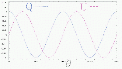
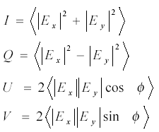
This graph shows how Q and U depend on the angle between the polarization vector and the x-axis. Since the polarization vector is invariant under rotation by 180 degrees, it is really only necessary to look at half of the plot. One sees that Q and U are out of phase by 45 degre
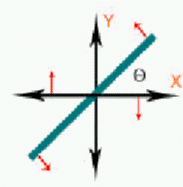
This image shows the definition of the angle Q used in the graph of Q and U. Note that the value of Q depends on both the polarization direction (shown by the bluish bar at an angle Q from the x-axis) and the orientation of the axes. The little red arrows on the axes and on the polarization vector point in the direction of increasing Q if the axes or the polarization vector were rotated.
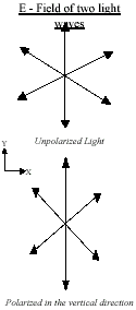
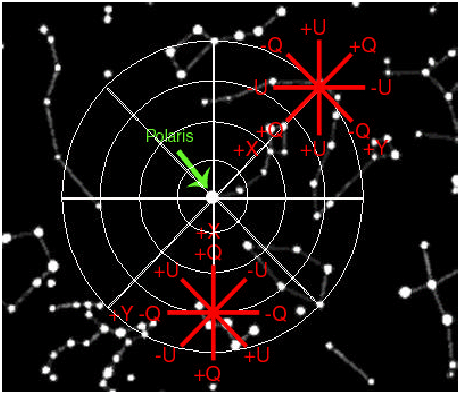
Which Way is Up?
IAU conventions define the axes used for polarization measurements. The x-axis points towards the North Celestial Pole, the point on the sky that is directly overhead at the Earth’s North Pole. The North Star, or Polaris, is very near to this point on the sky. The y-axis is orthogonal to the x-axis; it is chosen so that in a right handed coordinate system, the z-axis points from the point on the sky to the observer as shown in the picture on the right. The polarization directions in which Q and U are maximized or minimized are also shown; for example, if there is a +Q next to a line, then Q is maximized when the polarization direction is along that line. (Night sky background from http://www.emit.org/nightsky.html).
What are E- and B-modes? If you think of the vector field
for a static electric field, it has the interesting characteristic
that its curl is always zero. If you look
at a vector field for a static magnetic field, the divergence is
zero. In fact, one can break a vector field down
into components -- one with zero curl and one with zero divergence. In a similar way, we can break
down the polarization tensor field into two components, which
we call E and B modes. We liken E-modes to
a field with zero curl (like the static electric field), and B-modes
to a field with zero divergence (like the static magnetic field),
although technically divergence and curl are not defined on this
tensor field. (This has to do with the fact that
the polarization tensors don’t point in a unique direction). Appropriate
combinations of derivatives are used to define operations analagous
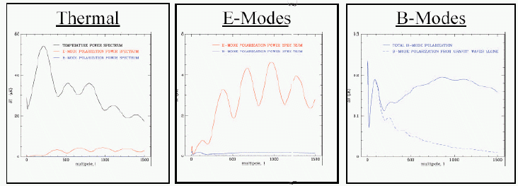
to divergence and curl. Most CMB polarization is in
the form of E-modes. It is possible that
B-modes also exist, and could be generated by two sources. One source would be gravity waves resulting
from the the violent ripping of spacetime that is predicted by inflation,
a theory that has not been confirmed. The
other source is gravitational lensing -- or the bending of light
due to matter (including dark matter). Gravity
waves in the early universe show up as B-modes on large angular
scales, while the gravitational lensing effects show up on smaller
scales (because the lensing is done by clusters, which are smaller). Finding experimental evidence for gravity
waves in the early universe would be a monumental discovery, and
better understanding of gravitational lensing can help solve questions
about dark matter and dark energy in the post-last-scattering universe. These effects have as of yet not been detected, which
is actually good, because B-modes from both these sources are
expected to be small and none of the current experiments has come
close to the sensitivity needed to see them. The
figures below show predicted CMB power spectra. The
ordinate is temperature while the abscissa is the ell of spherical
coordinates, a quantity roughly proportional to p/q, where q is the characteristic angular size
of fluctuations.
Before the surface of last
scattering, the universe was a hot plasma, with electrons and photons frantically
colliding. The CMB that we observe today is a snapshot
of the last light rays that scattered off this plasma just as it was cooling
enough for electrons to become bound in atoms. By
observing the properties of this light, we can draw conclusions about the
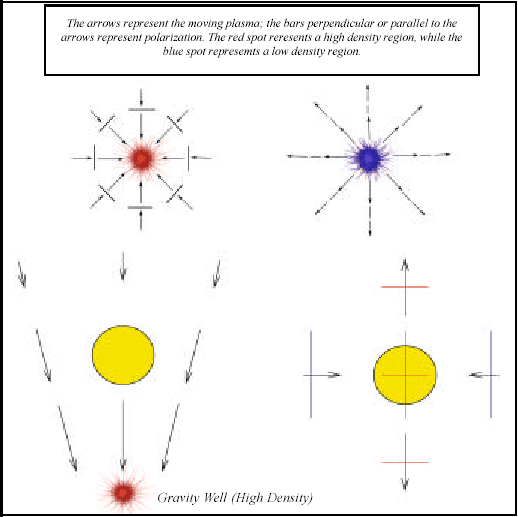
motion and densities of electrons (and other matter) at that time. A fascinating thing about polarization
in the CMB is that it gives us information about the velocity
of the plasma at the surface of last scattering.
Looking at the patterns of this motion can tell
us important information about the kind of oscillations that the
plasma was undergoing -- large-scale cosmic sound waves. The wavelength
of a sound wave could not exceed the size of the universe at the
time of the oscillation. Thus the
frequency spectrum of these sound waves provides information about the
expansion of the universe. Also, certain patterns
in the polarization, if present, could indicate the presence of gravity
waves in the early universe. The waves that categorize
these patterns are called “B-modes”, described in further detail above.
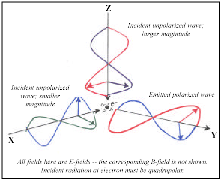
How Polarization is Made

Last
updated 8/4/03 If
you are having problems viewing this page, try this alternative
version. |
|||||||