Next: Observation log for June-July Up: thesis Previous: Summary Contents
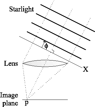 |
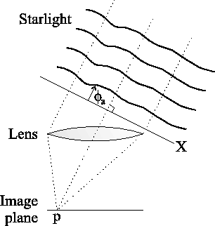
Figure A.2 shows the same situation as
Figure A.1, but the incoming wavefronts have been
perturbed by the atmosphere. The phase fluctuations will affect the
integral of the wavefunction over plane ![]() altering the measured
intensity at point
altering the measured
intensity at point ![]() .
.
 |
For the case of a single wind-blown Taylor screen, the phase
perturbations introduced by the atmosphere will be translated
laterally across the telescope aperture by the wind with no change in
the structure of these perturbations. The modulus of the integral of
the wavefunction over the plane ![]() is not directly affected by the
lateral motion of the phase fluctuations, but the motion of the screen
introduces new phase perturbations at the upwind side of the aperture
and removes phase perturbations at the downwind side. This can be seen
clearly if the outline of the telescope aperture is projected along
the line of sight from
is not directly affected by the
lateral motion of the phase fluctuations, but the motion of the screen
introduces new phase perturbations at the upwind side of the aperture
and removes phase perturbations at the downwind side. This can be seen
clearly if the outline of the telescope aperture is projected along
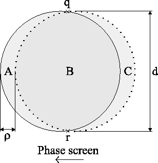
the line of sight from ![]() onto the Taylor screen, as shown by the
solid circle in Figure A.3. After time has elapsed
and the wind-blown Taylor screen has moved a distance
onto the Taylor screen, as shown by the
solid circle in Figure A.3. After time has elapsed
and the wind-blown Taylor screen has moved a distance ![]() , the
outline of telescope aperture will be projected onto the dotted
circle. Area
, the
outline of telescope aperture will be projected onto the dotted
circle. Area ![]() is common to both timepoints and will contribute
equally to the amplitude of the wavefunction at point
is common to both timepoints and will contribute
equally to the amplitude of the wavefunction at point ![]() in the image
plane, but the contribution from area
in the image
plane, but the contribution from area ![]() will be lost, and a new
contribution from area
will be lost, and a new
contribution from area ![]() will be included at the later timepoint. In
reality, the atmospheric phase in areas
will be included at the later timepoint. In
reality, the atmospheric phase in areas ![]() and
and ![]() will remain
correlated to that in area
will remain
correlated to that in area ![]() over a region extending approximately
over a region extending approximately
![]() from the boundary of area
from the boundary of area ![]() , but for the particular case of
large diameter apertures this only has a small effect on our
calculations and will be neglected in this simple approximation.
, but for the particular case of
large diameter apertures this only has a small effect on our
calculations and will be neglected in this simple approximation.
 |
We can write the contributions ![]() ,
, ![]() and
and ![]() to the wavefunction at point
to the wavefunction at point ![]() from areas
from areas ![]() ,
, ![]() and
and ![]() respectively as:
respectively as:
where ![]() ,
, ![]() and
and ![]() describe the amplitudes
and
describe the amplitudes
and ![]() ,
, ![]() and
and ![]() the phases of these
contributions. If the linear dimensions of areas
the phases of these
contributions. If the linear dimensions of areas ![]() ,
, ![]() and
and ![]() in
Figure A.3 are much larger than
in
Figure A.3 are much larger than ![]() , then the
phases
, then the
phases ![]() ,
, ![]() and
and ![]() will not be correlated
with each other, as the structure function of
Equation 1.3 indicates that the typical phase
variation between points separated by distances much greater
will not be correlated
with each other, as the structure function of
Equation 1.3 indicates that the typical phase
variation between points separated by distances much greater ![]() will be many cycles in magnitude.
will be many cycles in magnitude.
If the linear dimensions of areas ![]() ,
, ![]() and
and ![]() are much larger
than
are much larger
than ![]() then the ensemble average amplitudes
then the ensemble average amplitudes
![]() ,
,
![]() and
and
![]() will be
proportional to the square root of the areas of
will be
proportional to the square root of the areas of ![]() ,
, ![]() and
and ![]() respectively. This can most clearly be seen if we imagine utilising a
telescope whose aperture has the same size and shape as one of these
three regions. The atmospheric seeing will generate an image with a
FWHM of approximately
respectively. This can most clearly be seen if we imagine utilising a
telescope whose aperture has the same size and shape as one of these
three regions. The atmospheric seeing will generate an image with a
FWHM of approximately ![]() regardless of the aperture size
and shape (as long as the aperture is much larger than
regardless of the aperture size
and shape (as long as the aperture is much larger than ![]() ), with
an average intensity proportional to the area of the aperture.
), with
an average intensity proportional to the area of the aperture.
As the phases ![]() ,
, ![]() and
and ![]() are not
correlated with each other, if the light from more than one of the
these regions is combined then the ensemble averages of the relevant
amplitudes must be added in quadrature to give the total amplitude. It
is useful to consider three ensemble average intensities
are not
correlated with each other, if the light from more than one of the
these regions is combined then the ensemble averages of the relevant
amplitudes must be added in quadrature to give the total amplitude. It
is useful to consider three ensemble average intensities
![]() ,
,
![]() and
and
![]() which describe the contributions from the areas
which describe the contributions from the areas ![]() ,
, ![]() and
and ![]() as
follows:
as
follows:
| (A.4) | |||
| (A.5) | |||
| (A.6) |
| (A.7) |
We are interested in the intensity ![]() produced at the first
timepoint when light from areas
produced at the first
timepoint when light from areas ![]() and
and ![]() is combined:
is combined:
| (A.8) |
| (A.9) |
| (A.10) | |||
| (A.11) |
The value of
![]() is directly dependent on
is directly dependent on
![]() . For non-zero values of
. For non-zero values of
![]() , the
fluctuations in the instantaneous intensities
, the
fluctuations in the instantaneous intensities ![]() and
and ![]() will be correlated, as both intensities include a contribution from
will be correlated, as both intensities include a contribution from
![]() . Conversely, if the value of
. Conversely, if the value of
![]() were
zero then the contribution
were
zero then the contribution ![]() would be zero, and fluctuations
in
would be zero, and fluctuations
in ![]() and
and ![]() would be completely uncorrelated. We are
interested in determining the size of the contribution
would be completely uncorrelated. We are
interested in determining the size of the contribution
![]() for which the correlation between fluctuations in
for which the correlation between fluctuations in ![]() and
and ![]() has dropped by a factor of
has dropped by a factor of ![]() . As the wavefront
components
. As the wavefront
components ![]() ,
, ![]() and
and ![]() are uncorrelated
Rayleigh distributions, this will be true when the ensemble average
intensity
are uncorrelated
Rayleigh distributions, this will be true when the ensemble average
intensity
![]() from area
from area ![]() contributes
contributes
![]() of the total intensity:
of the total intensity:
The intensity
![]() will obey
Equation A.12 when areas
will obey
Equation A.12 when areas ![]() and
and ![]() are related as
follows:
are related as
follows:
| (A.13) |
If the telescope aperture is described by a function
![]() such as the example case in
Equation 1.7, then area of overlap
such as the example case in
Equation 1.7, then area of overlap ![]() between two offset apertures comes directly from the autocorrelation of
this function
between two offset apertures comes directly from the autocorrelation of
this function
![]() :
:
| (A.14) |
For the simple case presented in Figure A.3 of a
filled circular aperture of diameter ![]() , the area of overlap
, the area of overlap ![]() can
be calculated geometrically. The line joining
can
be calculated geometrically. The line joining ![]() and
and ![]() in
Figure A.3 is a chord to both the dotted and filled
circles.
in
Figure A.3 is a chord to both the dotted and filled
circles. ![]() is constructed from two symmetric regions either side of
this chord, each having an area:
is constructed from two symmetric regions either side of
this chord, each having an area: