Normalising the short-timescale component of the autocorrelation

Early investigations of atmospheric timescales typically involved a single high-speed photometer positioned at a single point in the image plane of a telescope. The temporal autocorrelation of a time series of measurements from such a device (i.e. the convolution of the time series with itself) provides a useful time-domain representation of the variance of the photometric flux with time. The long-timescale component of the measured temporal autocorrelation is assumed by Scaddan & Walker (1978) to be separable from the short-timescale component. The long-timescale (low frequency) component varies essentially linearly over the region of the autocorrelation which is of interest to speckle imaging. The solid line in Figure 2.1 shows a schematic representation of a typical temporal autocorrelation curve. The long-timescale component is indicated by the dashed line. In order to remove the effect of the long-timescale component, a linear fit to this component is calculated over the region of the temporal autocorrelation which is of interest for speckle imaging. 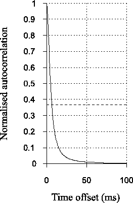The measured autocorrelation is then divided by this linear function to remove the long timescale component. The result can then be rescaled so that it ranges from zero to unity, to give the normalised high frequency component of the temporal autocorrelation as shown in Figure 2.2. The atmospheric timescale is the time delay over which this function decays to $1/e$, defined by Roddier et al. (1982a); Vernin et al. (1991) as $\tau _{e}$ (but known as $\tau_{1/e}^{B}$ in Scaddan & Walker (1978)). In Figure 2.2, $\tau _{e}$ is marked by the crossing point between the solid curve and dashed horizontal line.

Figure 2.1: Temporal autocorrelation for photometric measurements at a fixed point (solid curve). The dashed line shows a linear fit to the long-timescale fluctuations brought about by motion of the image centroid.

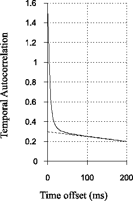Figure 2.2: Normalised temporal autocorrelation for photometric measurements at a fixed point (solid curve). The dashed line marks a value of $\frac{1}{e}$. The timescale $\tau _{e}$ is $7$ $ms$ in this example.