Timescales for exposure selection

A variation to the exposure selection method was developed in order to measure the timescale associated with the decorrelation of the brightest speckle in each exposure. The image selection and position corrections calculated for each exposure were actually applied to an earlier or later exposure. The exposure which was selected always came a fixed number of exposures before or after the exposure used for calculations of the Strehl ratio and position of the brightest speckle. For these analyses there thus exists a time difference between the measurement of the properties of the speckle pattern, and the response of the algorithm which selects and then co-adds the exposures. The analysis was repeated many times, varying the time difference used. No correction was made for the oscillation of the telescope, leaving an oscillation in the Strehl ratio as a function of the time difference used.

The Strehl ratio for the shift-and-add image using all the exposures is plotted as a function of this time difference in curve B of Figure 3.18, alongside curve A, the temporal autocorrelation of the speckle pattern previously shown in Figures 3.16 and 3.17. Qualitatively the curves appear similar suggesting that the decorrelation process is not substantially different for the brightest speckle than for the fixed point chosen in the image plane. Both curves are almost equally affected by the telescope oscillation as would be expected. If we ignore the effects of the telescope oscillation, the brightest speckle does appear to decorrelate slightly more quickly at first than the autocorrelation curve for the measurements taken at a fixed location in the image. Also shown in the Figure are the Strehl ratios obtained in the final image when the best $1$% of exposures are used, based upon the Strehl ratio and position of the brightest speckle measured in a different short exposure in the same run (i.e. taken at a slightly different time). If we ignore the effects of the telescope oscillation, this appears to decay slightly more slowly than the other timescales, perhaps indicating that the atmospheric coherence time is slightly extended during the times of the best exposures. This is a small effect, and it is clear that the timescales for the decay of the brightest speckle are very close to the coherence timescale of the speckle pattern.

Figure 3.18: Curve A shows the temporal autocorrelation of flux measurements at a single point in the image plane for the $\epsilon$ Aquilae data. Curves B and C show normalised plots of the Strehl ratio obtained when individual exposures are re-centred based on the measured position of the brightest speckle in a different exposure (with the time difference between the position measurement and the re-centring process indicated on the horizontal axis). All of the exposures in the run on $\epsilon$ Aquilae were used for curve B. For curve C, exposure selection and re-centring was based on the Strehl ratio and position of the brightest speckle in a different exposure, with only $1\%$ of the exposures selected.

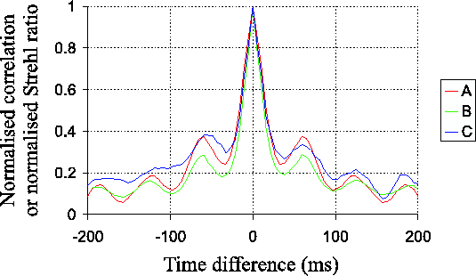Figure 3.18 shows that the timescale for the decay of the brightest speckle is $10$--$20$ $ms$ brought about predominantly by the $16$ $Hz$ telescope oscillation. If exposure times greater than this are used, one would expect the typical Strehl ratios of the exposures to be reduced. This was tested experimentally by splitting the dataset on $\epsilon$ Aquilae into groups of five consecutive exposures. The five exposures in each group were added together without re-centring to form a single exposure with five times the duration. The best $1$% of these $27$ $ms$ exposures is shown as a contour plot in Figure 3.19b alongside the shift-and-add image from the best $1$% of the original $5.4$ $ms$ exposures in Figure 3.19a. The increase in exposure time from $5.4$ $ms$ to $27$ $ms$ brings about a reduction in the Strehl ratio of the best $1$% from $0.26$ for Figure 3.19a to $0.22$ for Figure 3.19b. The image FWHM is increased from $79\times 94$ $mas$ to $81\times96$ $mas$. It is clear that the amplitude of the telescope oscillation is small enough that relative good image quality can still be obtained with exposure times as long as $27$ $ms$ using the Lucky Exposures method.

Figure 3.19: a)--d) Image quality of $\epsilon$ Aquilae using differing criteria for exposure selection from a $32$ $s$ run. Contour levels are at $1$, $2$, $4$, $8$, $16$, $30$, $50$, $70$, $90\%$ peak intensity.

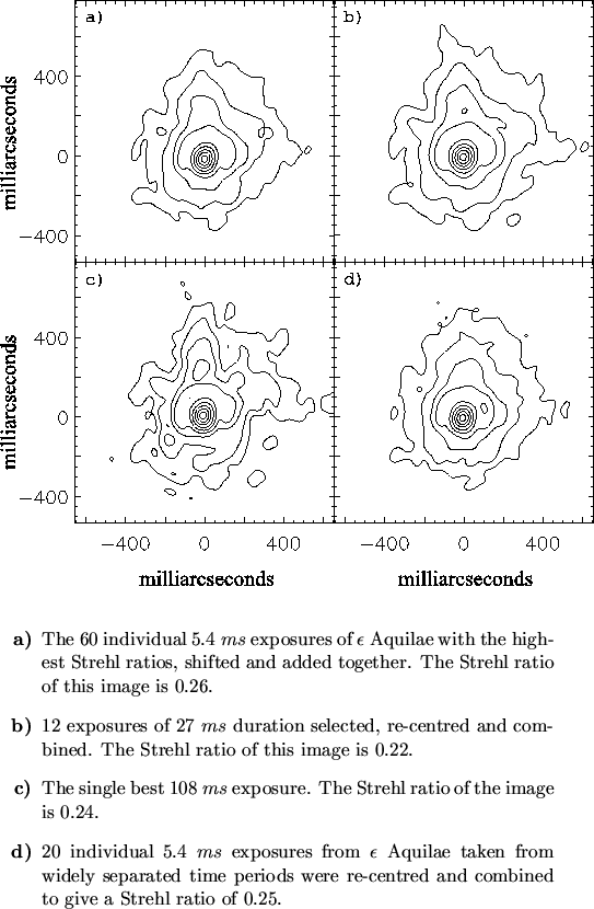Figure 3.19c shows the single best $108$ $ms$ exposure formed by summing together without re-centring $20$ consecutive short exposures from the run on $\epsilon$ Aquilae. The Strehl ratio for this image is $0.24$. The small amplitude of the telescope oscillation seen in movies generated from the raw short exposures around the moment that the $20$ constituent short exposures were taken may partly explain the high Strehl ratio obtained. It is clear that the atmospheric timescale must have been quite long at the time this exposure was taken. Although the Strehl ratios are comparable, the shift-and-add images shown in Figures 3.19a and 3.19b show much less structure in the wings of the PSF than the single exposure of Figure 3.19c. This is probably due to the shift-and-add images being the average of many atmospheric realisations, which helps to smooth out the fluctuations in the wings of the PSF. To demonstrate that this is not simply an integration-time effect, Figure 3.19d shows a shift-and-add image with the same total integration time and similar Strehl ratio ($0.25$) to Figure 3.19c, but using individual short exposures taken at widely separated times. The wings of the PSF are substantially smoother than for the $108$ $ms$ single exposure of Figure 3.19c. This suggests that a significant fraction of the noise in these images results from the limited number of atmospheric realisations used in generating them.