Next: Timescales for exposure selection Up: Observational results with single Previous: Exposure selection results Contents
In order to minimise the effects of long-timescale drift in the
location of the stellar PSF on the measurements, the pixel located at
the centroid of the long exposure average image of the run on
![]() Aquilae was selected (i.e. the centroid of
Figure 3.14d). The average image for this run had an
unusually compact PSF, showing no evidence for substantial drift in
the location of the speckle pattern during the
Aquilae was selected (i.e. the centroid of
Figure 3.14d). The average image for this run had an
unusually compact PSF, showing no evidence for substantial drift in
the location of the speckle pattern during the ![]()
![]() run. The
stellar flux from the selected pixel was recorded in each short
exposure, producing a one-dimensional dataset characterising the
temporal fluctuations in the PSF. The temporal power spectrum of this
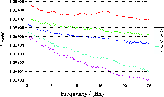
dataset is shown as curve A in Figure 3.15. The
power spectrum shows a peak at a frequency of
run. The
stellar flux from the selected pixel was recorded in each short
exposure, producing a one-dimensional dataset characterising the
temporal fluctuations in the PSF. The temporal power spectrum of this
dataset is shown as curve A in Figure 3.15. The
power spectrum shows a peak at a frequency of ![]()
![]() . This is in
close agreement with the first harmonic of mechanical oscillation for
the telescope structure, and movies made from the raw speckle images
clearly show motion consistent with such oscillations. The frequency
was confirmed to be
. This is in
close agreement with the first harmonic of mechanical oscillation for
the telescope structure, and movies made from the raw speckle images
clearly show motion consistent with such oscillations. The frequency
was confirmed to be ![]()
![]() by measuring the position of the
brightest speckle in each short exposure and then looking at the
temporal power spectrum of this time series.
by measuring the position of the
brightest speckle in each short exposure and then looking at the
temporal power spectrum of this time series.
 |
The effect of telescope oscillation on the temporal fluctuations at a
fixed point in the image plane can be seen by splitting into partial
derivatives the derivative of the flux ![]() with respect to time at a
fixed point in the telescope image plane. It is simplest to work in a
coordinate frame which is fixed with respect to the speckle pattern,
and study the effect of moving the optical detector at a velocity
with respect to time at a
fixed point in the telescope image plane. It is simplest to work in a
coordinate frame which is fixed with respect to the speckle pattern,
and study the effect of moving the optical detector at a velocity
![]() relative to the speckle pattern. In these coordinates,
the time derivative of the flux is:
relative to the speckle pattern. In these coordinates,
the time derivative of the flux is:
It is the total differential from
Equation 3.3 which limits the exposure time
we can use during observations at the NOT. For our data it is the
telescope oscillation which provides the dominant contribution on
short timescales. If the amplitude of the telescope oscillation could
somehow be reduced however, the ultimate limit to the exposure time
would be set by the partial derivative
![]() . This term represents the component of the
time variation in the flux which is introduced directly by changes in
the speckle pattern. It is of interest to try to measure the timescale
associated with this, as it would be applicable to other telescopes
operating under similar atmospheric conditions.
. This term represents the component of the
time variation in the flux which is introduced directly by changes in
the speckle pattern. It is of interest to try to measure the timescale
associated with this, as it would be applicable to other telescopes
operating under similar atmospheric conditions.
Curve A in Figure 3.16 shows the temporal
autocorrelation of the same dataset from ![]() Aquilae as
Figure 3.15 (it represents the Fourier transform
of curve A in Figure 3.15). The curve has been
normalised so that it ranges from unity at zero time difference to a
mean value of zero for time differences between
Aquilae as
Figure 3.15 (it represents the Fourier transform
of curve A in Figure 3.15). The curve has been
normalised so that it ranges from unity at zero time difference to a
mean value of zero for time differences between ![]()
![]() and
and
![]()
![]() . The
. The ![]()
![]() oscillatory component is clearly
visible. This oscillation is largely responsible for the initial
decorrelation in the measured flux as a function of time. The
telescope oscillation will only reduce the temporal correlation, so
the true autocorrelation function corresponding to the atmosphere
would lie above curve A for all time differences. The effect of
photon-shot noise was negligible in these observations due to the high
flux in each individual exposure. The frame rate (
oscillatory component is clearly
visible. This oscillation is largely responsible for the initial
decorrelation in the measured flux as a function of time. The
telescope oscillation will only reduce the temporal correlation, so
the true autocorrelation function corresponding to the atmosphere
would lie above curve A for all time differences. The effect of
photon-shot noise was negligible in these observations due to the high
flux in each individual exposure. The frame rate (![]()
![]() ) was
sufficiently high that the sharp peak in curve A around zero time
difference is relatively well sampled in this dataset (the peak does
not simply correspond to a single high value at zero time difference,
but contains several data points).
) was
sufficiently high that the sharp peak in curve A around zero time
difference is relatively well sampled in this dataset (the peak does
not simply correspond to a single high value at zero time difference,
but contains several data points).
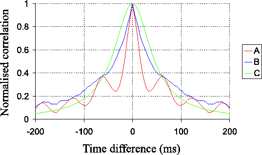 |
Curve B in this Figure is a function extrapolated from the measured
curve by dividing it by a decaying sinusoid having the same period as
the telescope oscillation. The amplitude and decay time of the
sinusoid were chosen so as to minimise the residual component at
![]()
![]() . This curve is intended to represent a possible shape for
the temporal autocorrelation in the absence of telescope oscillation.
. This curve is intended to represent a possible shape for
the temporal autocorrelation in the absence of telescope oscillation.
Curve C shows a fit to curve B of the form of Equation 2.2 (based on the model of temporal fluctuations by Aime et al. (1986)). The broad peak produced by this model does not seem consistent with the sharp peak seen in the experimental data.
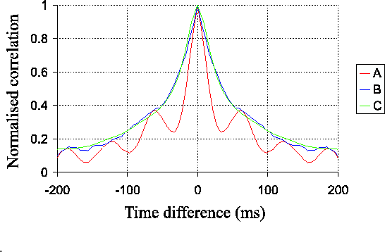
The sharp peak seen in curves A and B of
Figure 3.16 could be reproduced qualitatively
in numerical simulations if multiple Taylor screens were used with a
scatter of different wind velocities. One example of a simulation
which gave a better fit to the shape of the experimentally measured
temporal autocorrelation is shown as curve C in
Figure 3.17. The atmospheric model for this
simulation consisted of two Taylor screens moving at constant
velocities. Both layers moved in the same direction but with different
speeds. One layer, containing ![]() of the the turbulence took
of the the turbulence took
![]()
![]() to cross the diameter of the telescope aperture. The other
contained
to cross the diameter of the telescope aperture. The other
contained ![]() of the turbulence, but took only
of the turbulence, but took only ![]()
![]() to cross
the telescope aperture. Curves A and B from
Figure 3.16 are also reproduced as curves
A and B in Figure 3.17 for
comparison. Temporal power spectra generated using this model of the
atmosphere are plotted as curves B and C in
Figure 3.15. It is clear that they provide a much
better fit to the experimentally measured data in curve A
than the single layer atmospheric models shown in curves
D and E.
to cross
the telescope aperture. Curves A and B from
Figure 3.16 are also reproduced as curves
A and B in Figure 3.17 for
comparison. Temporal power spectra generated using this model of the
atmosphere are plotted as curves B and C in
Figure 3.15. It is clear that they provide a much
better fit to the experimentally measured data in curve A
than the single layer atmospheric models shown in curves
D and E.
 |
It is clear from the temporal autocorrelation plots of
Figures 3.16 and 3.17 that
there are (at least) two timescales associated with the decorrelation
of the speckle pattern: the half-period of the telescope oscillation
and the timescale for the decorrelation of the atmosphere. The
decorrelation timescale ![]() (as defined in
Chapter 2.2.1) which results from the combination
of these two effects is
(as defined in
Chapter 2.2.1) which results from the combination
of these two effects is ![]()
![]() . Using a simple fit to the
oscillatory component (used to produce curve B in both
Figures) the decorrelation timescale for the atmosphere alone was
calculated to be
. Using a simple fit to the
oscillatory component (used to produce curve B in both
Figures) the decorrelation timescale for the atmosphere alone was
calculated to be ![]()
![]() .
.
If the atmosphere had a single, boiling-free layer then
Equation 2.14 could be used to obtain the wind
velocity. Taking ![]()
![]() (consistent with the seeing disk,
and with the Strehl ratios in
Figure 3.10), a wind velocity of
(consistent with the seeing disk,
and with the Strehl ratios in
Figure 3.10), a wind velocity of
![]()
![]()
![]() is obtained. This is significantly larger than the
wind velocity near ground level of
is obtained. This is significantly larger than the
wind velocity near ground level of ![]()
![]()
![]() (from
Figure 3.7), but would not be implausible if the
turbulence were situated at high altitude.
(from
Figure 3.7), but would not be implausible if the
turbulence were situated at high altitude.
If the atmosphere had multiple layers travelling at different
velocities, and the timescale for decorrelation of the wavefronts was
shorter than the wind crossing timescale of the telescope aperture,
then the dispersion in the wind velocities ![]() could be
calculated using
Equation 2.12. The value obtained for
could be
calculated using
Equation 2.12. The value obtained for
![]()
![]() is
is ![]()
![]()
![]() (again
taking
(again
taking ![]()
![]() ). This level of dispersion in wind velocities
between atmospheric layers seems consistent with the wind
velocity of
). This level of dispersion in wind velocities
between atmospheric layers seems consistent with the wind
velocity of ![]()
![]()
![]() measured near to the ground.
measured near to the ground.
Both of these atmospheric configurations are plausible. The second is perhaps more likely given that the strongest turbulence is most commonly found at relatively low altitudes, where small wind speeds were observed.
Bob Tubbs 2003-11-14