Application to observational data

Two stars were observed without saturation at the end of the first night of technical time at the NOT in May 2000, as listed in Table 3.2. The individual short exposures were sinc-resampled to have four times finer pixel sampling, and Strehl ratios for each of the exposures were calculated from the flux in the peak pixel of the resampled images using Equation 3.2. The value of the normalisation constant $C$ used was $8573$ $mas^{2}$ calculated from the peak pixel value in simulations of diffraction-limited PSFs pixellated in the same way as the CCD observations. A summary of the results of this analysis including a histogram of the Strehl ratios for the run on $\epsilon$ Aquilae was included in Baldwin et al. (2001).

The Strehl ratios calculated in this way provide a direct comparison between the peak flux in the sinc-resampled short exposures with the peak flux which would be expected in a diffraction-limited exposure taken with the same camera. The sinc-resampling process produces a small change in the peak pixel flux in the short exposure images (typically $10$%) which leads to the slightly unsatisfactory situation that simulated short exposures under diffraction-limited atmospheric conditions processed in the same way give Strehl ratios greater than unity (the sinc-resampled images have a higher peak flux than the non-resampled images). This was resolved by recalculating the constant $C$ based upon the peak flux in diffraction-limited PSFs which had been sinc-resampled in the same way as the observational data. The value of $C$ is reduced from $8573$ $mas^{2}$ to $7060$ $mas^{2}$ in this case, causing a proportionate decrease in the estimated Strehl ratios. The Strehl ratios presented in this thesis were all calculated using the reduced value of $C$, giving values which are slightly smaller than those quoted in Baldwin et al. (2001).

The Strehl ratios calculated for the individual short exposures of $\epsilon$ Aquilae were binned into a histogram, and this is plotted alongside similar histograms calculated for a number of numerical simulations in Figure 3.10. It was possible to select atmospheric seeing conditions for each model which led to good agreement between the model Strehl histograms and those for the run on $\epsilon$ Aquilae. The four curves in the figure show:

A.

a numerical simulation with mirror perturbations described by model $1$ (those measured by Sørensen (2002)) and an atmosphere having $r_{0}$ five times smaller than the telescope diameter;

B.

a simulation using the mirror perturbations described by model $2$ (with large scale structure removed) with an atmosphere having $r_{0}$ seven times smaller than the telescope diameter;

C.

a simulation using model $3$, a diffraction-limited telescope with an atmosphere having $r_{0}$ eight times smaller than the telescope diameter; and

D.

the observations of $\epsilon$ Aquilae.

Figure 3.10: Simulated Strehl ratio histograms and measured data from the star $\epsilon$ Aquilae. Curves A, B and C correspond to models 1, 2 and 3 respectively (see Table 3.1). Atmospherically degraded short exposures were generated by combining Kolmogorov-like phase perturbations with those in the model used for the telescope aperture. The coherence length $r_{0}$ used for the Kolmogorov turbulence was $5$ times, $7$ times and $8$ times smaller than the telescope diameter for Curves A, B and C respectively. Curve D corresponds to a histogram of the measured Strehl ratios from short exposure images of $\epsilon$ Aquilae. Curves A, B and C have been re-scaled vertically to account for the difference between the number of simulated short exposures and the number of exposures taken on $\epsilon$ Aquilae (so the area under the four curves is the same).

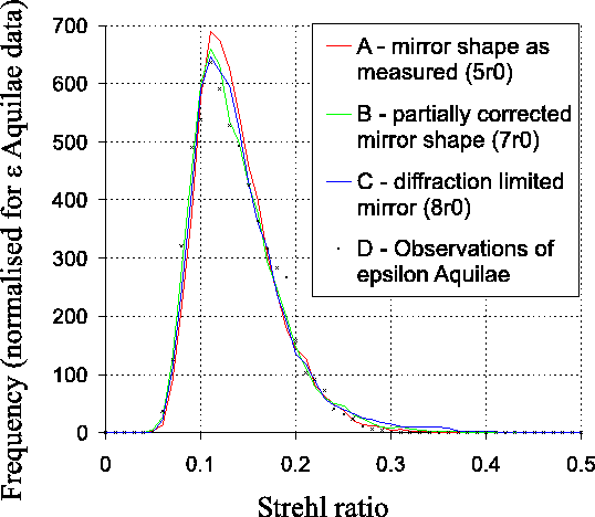The mirror perturbations on the NOT primary mirror are likely to have similar magnitude to those described by model $2$, implying that the most likely value for the atmospheric coherence length $r_{0}$ is $\frac{d}{7}$ or about $0.37$ $m$.

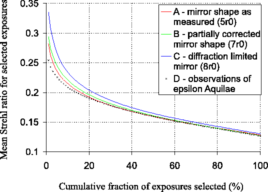
Figure 3.11 shows cumulative plots of the Strehl ratio datasets used in Figure 3.10. The exposures in each dataset were first sorted by descending Strehl ratio. Plotted in the figure for each dataset is the mean of the highest $1\%$ of Strehl ratios, the mean of the highest $2\%$ of Strehl ratios, and so on up to the mean of all the Strehl ratios in the dataset. These mean Strehl ratios give an indication of the image quality which would be obtained if a given fraction of exposures was selected for use in the Lucky Exposures method.

Figure 3.11: Cumulative Strehl ratio plots for the data presented in Figure 3.10. Curves A, B and C correspond to models 1, 2 and 3 respectively (as for Figure 3.10). The exposures having the highest Strehl ratios were selected from each dataset, and the mean of the Strehl ratios for the selected exposures is plotted against the total fraction of exposures selected (ranging from the best $1\%$ to $100\%$ of the exposures). Curve D shows the same plot for the measured Strehl ratios from short exposure images of $\epsilon$ Aquilae.

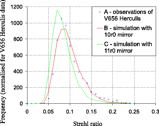
Strehl ratios were calculated in the same way for data taken on the star V656 Herculis, and Curve A in Figure 3.12 shows a histogram of the Strehl ratios obtained. Also shown in the figure are Strehl ratio histograms for simulations with a diffraction-limited telescope and atmospheric seeing conditions corresponding to $\frac{d}{r_{0}}=10$ (labelled B) and $\frac{d}{r_{0}}=11$ (labelled C). Again there is close correspondence between the simulated curves and the observational results. The lower Strehl ratios as compared to the run on $\epsilon$ Aquilae may result from slightly poorer seeing conditions, as highlighted by the long exposure FWHM in Table 3.2.

Figure 3.12: Strehl ratio histograms for the observation of V656 Herculis alongside two simulations. Curve A shows the Strehl ratios measured for V656 Herculis, curve B shows the Strehl ratio histogram for a simulation with a diffraction-limited mirror of $10r_{0}$ diameter, and curve C shows results of a simulation with an $11r_{0}$ diffraction-limited mirror. Curves B and C have been re-scaled vertically to account for the difference between the number of simulated short exposures and the number of exposures taken on V656 Herculis (so the area under the three curves is the same).