Data reduction method

In order to obtain a quantitive measure of the image quality, the Strehl ratio of the PSF in each short exposure was estimated from the flux in the brightest pixel in that exposure. Our estimate of the Strehl ratio of a short exposure was linearly related to the peak flux density $F_{p}$ in the image measured per steradian on the sky (calculated from the flux in the brightest pixel). This was divided by the total flux from the star in that exposure (integrated over the whole image: $\int_{-\infty}^{\infty}F\left ( \theta,\phi \right ) \mbox{d}\theta \mbox{d}\phi$). This gave an estimate $\mathcal{S}$ of the Strehl ratio:

$$\mathcal{S}=C\frac{F_{p}}{\int_{-\infty}^{\infty}F\left ( \theta,\phi \right ) \mbox{d}\theta \mbox{d}\phi}$$ (3.2)

The constant of proportionality $C$ represents a measure of the area of the PSF in steradians on the sky. In order to calculate the value of $C$ required to normalise the Strehl ratios for the case of diffraction-limited PSFs, it was necessary to generate a number of simulated PSFs.

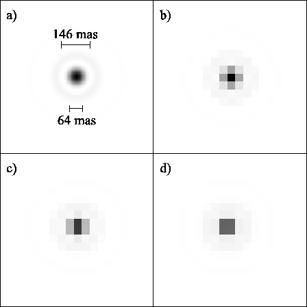
Simulated diffraction-limited PSFs were generated for the observing wavelength of $810$ $nm$ with flat incoming wavefronts at various tilt angles, using the aperture geometry described by Equation 3.1. An example is shown in Figure 3.8a. These were then binned into $41$ $mas$ pixels to match the camera resolution. The pixellated shape of the PSF was found to depend slightly on the tilt of the incoming wavefronts (i.e. the position of the PSF in relation to the pixel grid) as shown for three example PSFs in Figures 3.8b--d. This led to a variation of $\sim 15\%$ in the flux in the brightest pixel. Our estimate for the peak flux density was taken as the flux in the brightest pixel divided by the area of the pixel ($1681$ $mas^{2}$ for $41\times41$ $mas$ pixels). By setting the Strehl ratio of these diffraction-limited images to unity, values of $C$ were calculated from Equation 3.2. The mean value of $C$ for a grid of $32\times 32$ different wavefront tilts was calculated as $2.015\times10^{-13}$  $steradians^{2}$ ($8573$ $mas^{2}$).

Figure 3.8: a) Simulation of a diffraction-limited PSF for an aperture similar to that of the NOT (the precise aperture geometry used for the simulation is described by Figure 3.4). b)--d) demonstrate the pixel sampling of the PSF by our camera. The three images correspond to three different positions of the PSF with respect to the detector pixel grid. The pixels corresponded to $41$ $mas$ squares on the sky. The peak pixel in b)--d) typically contains $20\%$ of the light in the image.

In order to investigate the accuracy of Strehl ratio measurements on realistic PSFs, numerical simulations of observations were undertaken using Kolmogorov atmospheres where the incident flux in the image plane was integrated over individual $41\times41$ $mas$ pixels in a square array, again resembling the optical layout for the camera and CCD detector at the NOT. Strehl ratios for the individual short exposures were calculated from the flux in the brightest pixel as described above. The flux in the brightest pixel was found to vary at the $\sim 15$% level depending on sub-pixel variations in the position of the brightest speckle relative to the grid of pixels, in a similar manner to the case of the diffraction-limited PSF shown in Figures 3.8b--d. This implied a position dependent error in the measured Strehl ratio at the $15$% level (similar to the case for a diffraction-limited PSF).

So as to reduce the dependence of the measured Strehl ratio on the position of the stellar image on the CCD pixel array, the simulated short exposure images of the star were sinc-resampled to give four times finer pixel sampling in each coordinate. This was performed in the Fourier domain - the dimensions of the discrete Fourier domain were increased by padding it with zeros, and the power at Nyquist Fourier components was distributed equally at both positive and negative frequencies. The sinc-resampling process preserves the Fourier components with spatial frequencies below the Nyquist cutoff, and does not introduce any power at spatial frequencies above this cutoff. The Nyquist cutoff for the pixel sampling of the CCD in the horizontal and vertical directions of $12$ $cycles$ $as^{-1}$ is only slightly lower than highest spatial frequency components in the PSF of around $\frac{d}{\lambda}=15$ $cycles$ $as^{-1}$ (in other words only a small range of spatial frequencies are not adequately sampled by the CCD). Spatial frequency components of the PSF above the Nyquist cutoff for the CCD pixel sampling are expected to contain little power, making the sinc-resampled short exposures a reasonably good approximation to the original PSF before the pixellation process (although spatial frequencies just below the Nyquist cutoff of the CCD array will be suppressed due to the finite pixel size). The four-fold sinc-resampling process successfully reduced the variation in Strehl ratio with image position to $1\%$ or less. Further resampling with even finer pixel spacing had little effect on the measured Strehl ratios.

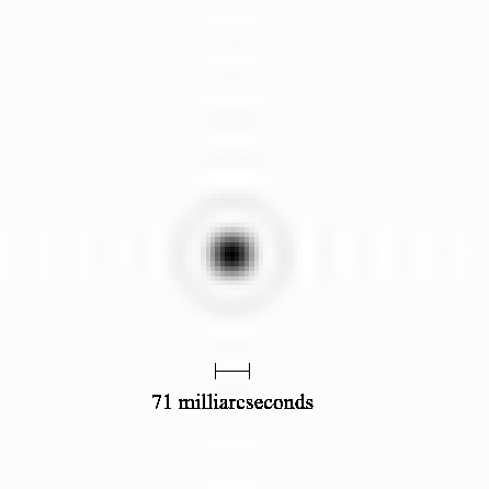
The ability of the sinc-resampling process to recreate the original PSF is demonstrated in Figure 3.9. In this Figure, diffraction-limited PSFs with a range of different position offsets were pixellated in the same way as was shown in Figures 3.8b--d. The pixellated images were then sinc-resampled with four times as many pixels in both dimensions, and the resulting images were shifted to a common centre and co-added to form Figure 3.9. The Airy pattern is clearly reproduced, and the FWHM of the image core is only slightly larger than that for the true diffraction-limited PSF shown in Figure 3.8a. The sinusoidal ripples extending in both the horizontal and vertical directions from the core of Figure 3.9 are a result of aliasing (Gibb's phenomenon), as the Nyquist cutoff for the CCD pixel sampling in the horizontal and vertical directions is slightly less than the highest spatial frequency $\frac{d}{\lambda}$ (the Nyquist cutoff frequency is sufficiently high along the image diagonal that aliasing does not occur).

Figure 3.9: A PSF reconstructed from pixellated exposures using sinc-resampling and image re-centring. The NOT PSF was sampled with $41$ $mas$ square pixels at a grid of $32\times 32$ different sub-pixel positions similar to (and including) those shown in Figure 3.8. The resulting images were sinc-resampled to have four times as many pixels in each dimension, and shifted and added together using the location brightest pixel in the resampled image for re-centring.