Next: Observations Up: Experimental method Previous: Background Contents
In order to investigate the possible impact of any remaining aberrations, I undertook simulations with various different levels of mirror aberration. In the absence of direct measurements of the mirror shape after the adjustment to the actuators had been made I have suggested two models for the mirror aberrations as follows:
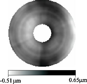
Model 1 represents a ``worst-case scenario'', with no improvement to the mirror aberrations after adjustment of the mirror supports. The mirror aberrations are taken directly from measurements of wavefront curvature made before the mirror actuators were adjusted (these measurements were provided by Sørensen (2002)). There is no defocus component in the model. The wavefront errors are shown as a function of position in the aperture plane in Figure 3.2.
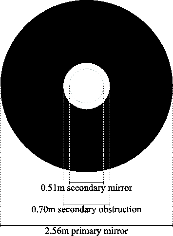
Model 2 is identical to model 1 except that mirror aberrations on scales larger than the mean separation between adjacent mirror supports have been strongly suppressed. It is intended to represent a ``best-case scenario'', with near-optimal corrections to the mirror supports. The wavefront errors for model 2 are shown in Figure 3.3. It is understood that the residual wavefront errors at the NOT were small after the mirror actuators had been adjusted, hence the real shape of the primary mirror was probably similar to that shown in model 2.
 |
Models 1 and 2 are intended to represent the two extremes of negligible improvement and near-optimal improvement. A third model investigated for purposes of comparison was that of a diffraction-limited mirror. The three models are summarised in Table 3.1
For each of the models the telescope PSF in the absence of the
atmosphere was generated using an FFT (as described in
Chapter 1.2.2). The PSF Strehl ratios obtained were
![]() ,
, ![]() and
and ![]() for models 1, 2 and 3 respectively.
for models 1, 2 and 3 respectively.
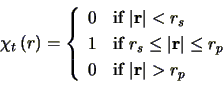
For the numerical simulations based upon these models, the secondary
supports were ignored, and the telescope aperture was modelled as an
annulus with inner radius ![]() equal to that of the secondary
obscuration, and outer radius
equal to that of the secondary
obscuration, and outer radius ![]() determined by the radius of the
primary mirror (as shown in Figure 3.4). The
shape of the aperture used in the simulations can be described
mathematically in terms of the throughput
determined by the radius of the
primary mirror (as shown in Figure 3.4). The
shape of the aperture used in the simulations can be described
mathematically in terms of the throughput
![]() as a function of radius
as a function of radius ![]() (in the same way as for
Equation 1.7):
(in the same way as for
Equation 1.7):
For each model, many realisations of atmospheric phase fluctuations
that had a Kolmogorov distribution with ![]() seven times smaller
than telescope diameter were calculated. These Kolmogorov
distributions had a large outer scale (approximately thirty times the
telescope diameter). The phase perturbations from the telescope mirror
for each model were added to the simulated atmospheric phase
distribution, and short exposure images were generated using the
aperture shape described by
Equation 3.1. The mirror aberrations in
models
seven times smaller
than telescope diameter were calculated. These Kolmogorov
distributions had a large outer scale (approximately thirty times the
telescope diameter). The phase perturbations from the telescope mirror
for each model were added to the simulated atmospheric phase
distribution, and short exposure images were generated using the
aperture shape described by
Equation 3.1. The mirror aberrations in
models ![]() and
and ![]() produce a reduction in the typical Strehl ratios
for the short exposure images when compared with the
diffraction-limited case. Histograms showing the frequency
distribution of Strehl ratios measured for the short exposures from
each of the models are shown in Figure 3.5.
produce a reduction in the typical Strehl ratios
for the short exposure images when compared with the
diffraction-limited case. Histograms showing the frequency
distribution of Strehl ratios measured for the short exposures from
each of the models are shown in Figure 3.5.
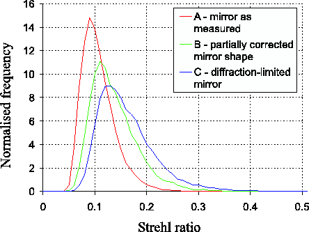 |
It is interesting to note that with model ![]() (the worst-case
scenario) some of the short exposures through the atmosphere have
higher Strehl ratios than would be obtained in the absence of the
atmosphere. In these exposures the atmospheric phase perturbations are
compensating for the errors in the figure of the telescope
mirror. This effect is even more noticeable under slightly better
astronomical seeing conditions. One example of an exposure with very
high Strehl ratio which appeared by chance in such a simulation is
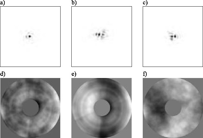
shown in Figures 3.6a--f.
(the worst-case
scenario) some of the short exposures through the atmosphere have
higher Strehl ratios than would be obtained in the absence of the
atmosphere. In these exposures the atmospheric phase perturbations are
compensating for the errors in the figure of the telescope
mirror. This effect is even more noticeable under slightly better
astronomical seeing conditions. One example of an exposure with very
high Strehl ratio which appeared by chance in such a simulation is
shown in Figures 3.6a--f. ![]() for this
simulation was five times smaller than the telescope diameter.
Figure 3.6a shows the selected exposure with a
Strehl ratio of 0.32. The PSF of the telescope (in the absence of
atmospheric perturbations) is shown in
Figure 3.6b, with a Strehl ratio of
0.23. Figure 3.6c shows the PSF that would be
obtained through the same atmosphere using a diffraction-limited
telescope (i.e. the PSF for the atmospheric perturbations alone). The
shape of this PSF is almost a mirror-image of
Figure 3.6b, suggesting that the wavefront errors
from the atmosphere are approximately equal and opposite to the
aberrations introduced by the telescope. This is also apparent in
Figures 3.6d, 3.6e and
3.6f which show greyscale maps of the wavefront
error for the PSFs in Figures 3.6a,
3.6b and 3.6c respectively.
for this
simulation was five times smaller than the telescope diameter.
Figure 3.6a shows the selected exposure with a
Strehl ratio of 0.32. The PSF of the telescope (in the absence of
atmospheric perturbations) is shown in
Figure 3.6b, with a Strehl ratio of
0.23. Figure 3.6c shows the PSF that would be
obtained through the same atmosphere using a diffraction-limited
telescope (i.e. the PSF for the atmospheric perturbations alone). The
shape of this PSF is almost a mirror-image of
Figure 3.6b, suggesting that the wavefront errors
from the atmosphere are approximately equal and opposite to the
aberrations introduced by the telescope. This is also apparent in
Figures 3.6d, 3.6e and
3.6f which show greyscale maps of the wavefront
error for the PSFs in Figures 3.6a,
3.6b and 3.6c respectively.
 |
The atmosphere is much less likely to correct those phase
perturbations which have small spatial scales across the telescope
mirror, because the Kolmogorov wavefront perturbations have very
little power on small spatial scales. The perturbations in model ![]() are restricted to small spatial scales so little correction is
expected, but the phase perturbations in the model are sufficiently
small in amplitude that they only have a small impact on the
distribution of the measured Strehl ratios, as shown in
Figure 3.5.
are restricted to small spatial scales so little correction is
expected, but the phase perturbations in the model are sufficiently
small in amplitude that they only have a small impact on the
distribution of the measured Strehl ratios, as shown in
Figure 3.5.
It is clear from the tails of the distributions in
Figure 3.5 that we can expect the best short
exposure images taken at the NOT to have reasonably high Strehl
ratios under good atmospheric seeing conditions. Even with model 1,
representing something of a worst-case scenario, Strehl ratios higher
than ![]() are expected
are expected ![]() of the time.
of the time.
Bob Tubbs 2003-11-14