The Kolmogorov model of turbulence

A description of the nature of the wavefront perturbations introduced by the atmosphere is provided by the Kolmogorov model developed by Tatarski (1961), based partly on the studies of turbulence by the Russian mathematician Andreï Kolmogorov (Kolmogorov, 1941a,b). This model is supported by a variety of experimental measurements (e.g. Colavita et al. (1987); Nightingale & Buscher (1991); Buscher et al. (1995); O'Byrne (1988)) and is widely used in simulations of astronomical imaging. The model assumes that the wavefront perturbations are brought about by variations in the refractive index of the atmosphere. These refractive index variations lead directly to phase fluctuations described by $\phi_{a} \left(\mathbf{r}\right)$, but any amplitude fluctuations are only brought about as a second-order effect while the perturbed wavefronts propagate from the perturbing atmospheric layer to the telescope. For all reasonable models of the Earth's atmosphere at optical and infra-red wavelengths the instantaneous imaging performance is dominated by the phase fluctuations $\phi_{a} \left(\mathbf{r}\right)$. The amplitude fluctuations described by $\chi_{a} \left(\mathbf{r}\right)$ have negligible effect on the structure of the images seen in the focus of a large telescope.

The phase fluctuations in Tatarski's model are usually assumed to have a Gaussian random distribution with the following second order structure function:

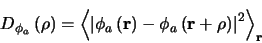$$D_{\phi_{a}}\left(\mathbf{\rho} \right) = \left \langle \lef... ...{\rho} \right ) \right \vert ^{2} \right \rangle _{\mathbf{r}}$$ (1.3)

where $D_{\phi_{a}} \left ({\mathbf{\rho}} \right )$ is the atmospherically induced variance between the phase at two parts of the wavefront separated by a distance $\mathbf{\rho}$ in the aperture plane, and $\left < \ldots \right >$ represents the ensemble average.

The structure function of Tatarski (1961) can be described in terms of a single parameter $r_{0}$:

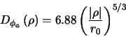$$D_{\phi_{a}} \left ({\mathbf{\rho}} \right ) = 6.88 \left ( ... ...\left \vert \mathbf{\rho} \right \vert}{r_{0}} \right ) ^{5/3}$$ (1.4)

$r_{0}$ indicates the ``strength'' of the phase fluctuations as it corresponds to the diameter of a circular telescope aperture at which atmospheric phase perturbations begin to seriously limit the image resolution. Typical $r_{0}$ values for I band ($900$ $nm$ wavelength) observations at good sites are $20$--$40$ $cm$. Fried (1965) and Noll (1976) noted that $r_{0}$ also corresponds to the aperture diameter for which the variance $\sigma ^{2}$ of the wavefront phase averaged over the aperture comes approximately to unity:

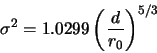$$\sigma ^{2}=1.0299 \left ( \frac{d}{r_{0}} \right )^{5/3}$$ (1.5)

Equation 1.5 represents a commonly used definition for $r_{0}$.

A number of authors (e.g. Mandelbrot (1974); Kuo & Corrsin (1972); Siggia (1978); Frisch et al. (1978); Kim & Jaggard (1988)) have suggested alternatives to this Gaussian random model designed to better describe the intermittency of turbulence discovered by Batchelor & Townsend (1949). Although variations in seeing conditions have been found on timescales of minutes and hours (Wilson, 2003; Racine, 1996; Vernin & Muñoz-Tuñón, 1998), no significant experimental evidence has been put forward which strongly favours any one of the intermittency models for the turbulence involved in astronomical seeing. The Gaussian random model is still the most widely used, and will be the principal model discussed in this thesis.