Short exposure optical imaging through the atmosphere
It is first useful to give a brief overview of the basic theory of optical
propagation through the atmosphere. In the standard classical theory,
light is treated as an oscillation in a field  . For
monochromatic plane waves arriving from a distant point source with
wave-vector
. For
monochromatic plane waves arriving from a distant point source with
wave-vector  :
:
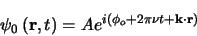 |
(1.1) |
where  is the complex field at position
  and
time
and
time  , with real and imaginary parts corresponding to the electric
and magnetic field components,
, with real and imaginary parts corresponding to the electric
and magnetic field components,  represents a phase offset,
 is the frequency of the light determined by
 , and
, and  is the
amplitude of the light.
is the
amplitude of the light.
The photon flux in this case is proportional to the square of the
amplitude , and the optical phase corresponds to the complex
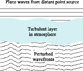
argument of . As wavefronts pass through the Earth's
atmosphere they may be perturbed by refractive index variations in the
atmosphere. Figure
1.2 shows schematically a turbulent layer in the
Earth's atmosphere perturbing planar wavefronts before they enter a
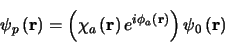
telescope. The perturbed wavefront  may be related at any
given instant to the original planar wavefront
may be related at any
given instant to the original planar wavefront
 in the following way:
 |
(1.2) |
where
 represents the fractional
change in wavefront amplitude and
represents the fractional
change in wavefront amplitude and
 is the change in wavefront phase introduced by the atmosphere. It is
important to emphasise that
and
describe the effect of the Earth's
atmosphere, and the timescales for any changes in these functions will
be set by the speed of refractive index fluctuations in the atmosphere.
is the change in wavefront phase introduced by the atmosphere. It is
important to emphasise that
and
describe the effect of the Earth's
atmosphere, and the timescales for any changes in these functions will
be set by the speed of refractive index fluctuations in the atmosphere.
Figure 1.2:
Schematic diagram illustrating how optical wavefronts from a
distant star may be perturbed by a turbulent layer in the
atmosphere. The vertical scale of the wavefronts plotted is highly
exaggerated.
 |
Subsections
Bob Tubbs
2003-11-14