Results using model 1 for the gain stages

Simulations of the CCD65 L3Vision device with $591$ gain stages were first undertaken using model 1 for the individual gain stages (where the additional impact ionisation electrons were chosen from a Poisson distribution). In the simulations the same value of the gain $\mu$ was used for each of the $591$ stages. The total gain of the multiplication register was thus given by $\mu^{591}$. The three simulations used three different values of $\mu$ chosen to give total multiplication register gains $g=\mu^{591}$ of $g=100$, $g=1000$ and $g=10000$. The probability distributions for the output electrons in these three simulations are shown in Figure 4.2.

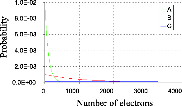
Figure 4.2: The probability distribution for the number of output electrons from a multiplication register of $591$ stages with a single electron input and total register gains of $100$, $1000$ and $10000$ (curves A, B and C respectively). All three probability curves fall to zero for the case of less than one output electron. For these simulations model 1 was used for the individual gain stages, where additional electrons are selected from a Poisson distribution. The same data are plotted on a logarithmic scale in Figure 4.3.

The probability distributions for the output electrons are well approximated by decaying exponential curves for large values of $n$. This is highlighted in Figure 4.3a where the curves are plotted on a logarithmic scale. The probability curves appear as straight lines over a wide range of $n$ in the plot. For very large values of $n$ the probability reaches the computational accuracy of the software corresponding to a value of $\sim10^{-16}$, and beyond this point the probability calculations are dominated by noise. Figure 4.3b shows an expanded view of the probability distributions for small $n$. Exponential curves were least-squares fitted to the probability curves for the large $n$ region, and these are extrapolated as dashed curves in this plot. For small values of $n$ ($n\ll\mu$) the probability curve begins to fall very slightly below the best fit exponential before dropping rapidly to zero for $n=0$.

Figure 4.3: The probability distributions from Figure 4.2 plotted on a logarithmic scale. A multiplication register of 591 stages was simulated with a single electron input and total register gains of 100, 1000 and 10000 (curves A, B and C respectively). Model 1 was used for the individual gain stages, where additional electrons are selected from a Poisson distribution. Panel b) shows an enlargement of one portion of the plot in panel a). The curves in panel a) were well fitted with exponential functions for the case of large numbers of output electrons, and these fits have been extrapolated as dashed lines in panel b).

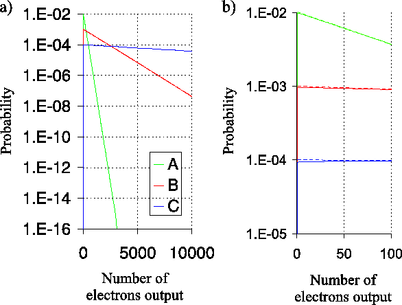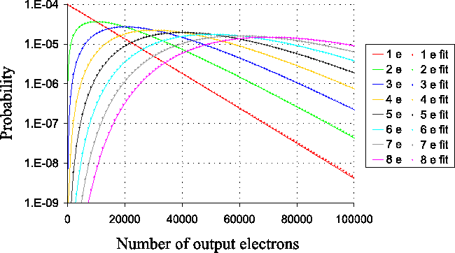
Figure 4.4 shows similar plots for a $591$ stage register with overall gain $g=1000$ with different numbers of input electrons. The general shape of the curves was not strongly dependent on the number of gain stages $s$ as long as $s$ was large.

Figure 4.4: The probability distribution for the number of output electrons from a multiplication register of $591$ stages with different numbers of input electrons. The discrete points on the graph show selected values from the numerical fit described by Equation 4.27, as discussed in the text.

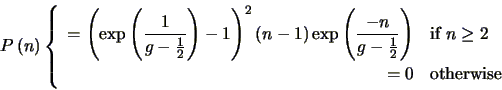
Based upon the exponential fits in Figure 4.3, we can say that the probability distributions for the number of output electrons produced when one input electron enters an electron multiplying CCD with a large number of gain stages can be approximated by the function:

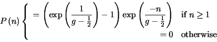$$P\left (n \right ) \left\{ \begin{array}{rl} \displaystyle... ...if $n\geq 1$} \\ = 0 & \mbox{otherwise} \end{array}\right.$$ (4.25)

where $n$ is an integer describing the number of output electrons and $g$ is the overall gain of the multiplication register.

If we approximate Equation 4.25 as a continuous function and convolve it with itself we get an approximation for the probability distribution given two input electrons:

$$P\left (n \right ) \left\{ \begin{array}{rl} \displaystyle... ...if $n\geq 2$} \\ = 0 & \mbox{otherwise} \end{array}\right.$$ (4.26)

With further convolutions, and taking approximations for the case of large gain $g$ and a large number $m$ of input electrons, I obtained the following model for the probability distribution for the output electrons:

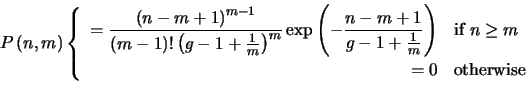$$P\left (n,m \right ) \left\{ \begin{array}{rl} \displaysty... ...{if $n\geq m$} \\ =0 & \mbox{otherwise} \end{array}\right.$$ (4.27)

where $n$ is the number of output electrons. Individual data points calculated using this equation are included in Figure 4.4 alongside the appropriate probability curves calculated numerically for model 1. The approximation described by Equation 4.27 does not differ substantially from the numerically calculated curves even for one or two input electrons (although slightly better approximations for one and two input electrons are given by Equations 4.25 and 4.26 respectively).