Results using model 2

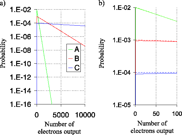
Figure 4.5 shows the probability distribution for the output electrons when the gain stages are described by model 2 (where electrons entering the gain stage can generate at most one electron by impact ionisation in that gain stage). The general shape of the curves is very similar to those produced by model 1 (see Figure 4.3 for comparison). With model 2 the curves fall away to zero slightly more quickly for small values of $n$. The approximations described by Equations 4.25 to 4.27 are also good descriptions for the output probability distributions with this model for the gain stages.

Figure 4.5: The probability distribution for the number of output electrons from a multiplication register of $591$ stages using model 2 for the gain stages with a single electron input to the register. With this model each electron input to one gain stage is only allowed to take part in one impact ionisation process within that stage. Curves A, B and C correspond to simulations with total gains of 100, 1000 and 10000. Panel b) shows an enlargement of one portion of the plot in panel a). The curves in panel a) were well fitted with exponential functions for the case of large numbers of output electrons, and these fits have been extrapolated as dashed lines in panel b).

It is perhaps not surprising that the probability distributions for the output electrons with the two different gain stage models considered here are so similar, given that it is the discretisation of the signal into individual electrons which dominates the signal-to-noise performance of the register, and not the internal properties of the individual gain stages. Even if the gain stages of a real multiplication register differ slightly from either of the models described above, it seems likely that Equation 4.25 will provide a good approximation to the distribution of output electrons given one input electron.