Example data from observations at the NOT

In order to provide an example of the camera performance achieved during observing runs at the NOT, I have included a small amount of data from the observing run in June 2003 in this Chapter.

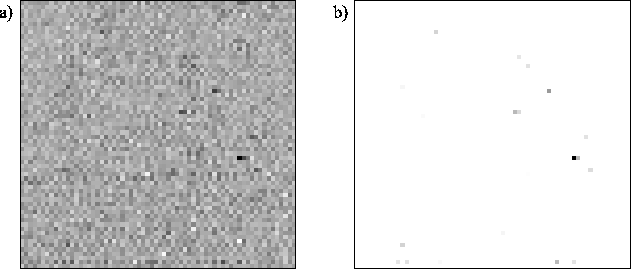
Figure 4.7 shows a small region of one short exposure taken while the camera was attached to the NOT on 2003 June 29. Long exposure imaging of the field displayed here showed that it did not contain any bright sources, so the detected flux is known to be much less than one photo-electron per pixel in this short exposure.

Figure 4.7: a) Part of a short exposure image taken at very low light level displayed as a negative image. b) The same negative image plotted with a greyscale having twice the contrast. Pixels with low signal levels have saturated to white with this greyscale.

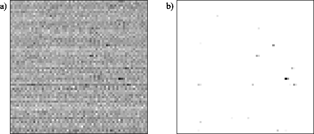A small number of pixels in the short exposure show signal levels which are significantly higher than the typical noise in the image. It is likely that a photo-electron (or dark current electron) was generated in most of these pixels. The pixels with high signal levels found in several thousand short exposures such as this were found to be correlated with the locations of faint sources in the field, suggesting that they do indeed correspond to photon events.

Figure 4.8 shows a histogram of the Digital Numbers (DNs) output from the camera in $5000$ exposures similar to the one shown in Figure 4.7 (and including the exposure shown). The peak of the histogram can be relatively well fit by a Gaussian distribution, as shown in Figure 4.8a. The centre of this Gaussian distribution corresponds to the mean signal when no photons are detected in a pixel. The width of the Gaussian corresponds to the RMS readout noise. A least-squares fit to the data gave a value of $2799.9$ $DN$ for the centre of the Gaussian. The fitted Gaussian dropped to $1/e$ of the peak value $5.81$ $DN$ from the centre, implying an RMS readout noise of $5.81$ $DN$. If each $DN$ corresponds to $a$ electrons leaving the multiplication register, the RMS readout noise $R$ will be:

$$R=5.81a\mbox{ electrons}$$ (4.30)

Figure 4.8: a) Histogram of the $DN$s measured by the CCD camera in $5000$ exposures similar to that shown in Figure 4.7. A Gaussian has been least-squares fitted to the data. b) The same histogram plotted on a logarithmic scale. An exponentially decaying function has been fit to the data for high $DN$s.

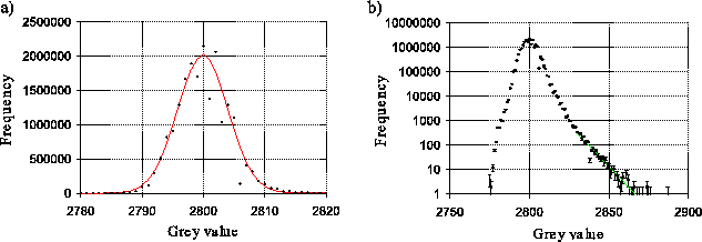Figure 4.8b shows the same measurement data plotted on a logarithmic scale. The frequency distribution is well fit by an exponentially decaying function for high $DN$s (more than $5R$ from the centre of the Gaussian) as would be expected given the presence of photo-electrons in some of the pixels. The best fit exponential had a decay constant of $-0.156$ per $DN$. The gain of the multiplication register can be calculated from Equation 4.25 as:

$$g=\frac{a}{0.156}+\frac{1}{2}$$ (4.31)

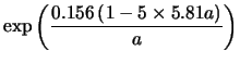
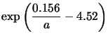
Applying Equation 4.29 to the parameters given by Equations 4.30 and 4.31 allows us to calculate the efficiency $f$ for counting photo-electrons:

$$f = \exp{ \left ( \frac{0.156\left (1-5\times5.81a \right )}{a} \right )}$$ (4.32)

$$= \exp{ \left ( \frac{0.156}{a} - 4.52 \right )}$$ (4.33)

For $a\gg0.156$ this gives an efficiency for photo-electron detection of:

$$f \simeq \exp{ \left ( - 4.52 \right )}$$ (4.34)

$$= 0.011$$ (4.35)

which is far too low to be of practical use. $a$ was expected to be approximately $100$ based on the electronic setup of the camera).

The reason for the poor photon counting performance is highlighted if the RMS readout noise is expressed in terms of the mean input signal provided by one photo-electron (i.e. if the RMS readout noise is expressed in units of photo-electrons). This is achieved if Equation 4.30 is divided by Equation 4.31:

$$R=\frac{5.81a}{a/0.156+1/2} \mbox{ photo-electrons}$$ (4.36)

As $a\gg0.156$ we can approximate this as:

$$R = 5.81\times0.156 \mbox{ photo-electrons}$$ (4.37)

$$= 0.906 \mbox{ photo-electrons}$$ (4.38)

Although the RMS readout noise is less than the mean signal from a photo-electron, it is too large to accurately distinguish most photon events from the readout noise.

It should be noted that a readout noise of $0.9$ photo-electrons at $3.5$ $MHz$ pixel rates represents a very substantial improvement over the read noise of $50$--$60$ electrons for the camera used in the observations described in Chapter 3. State-of-the-art conventional CCDs can typically only achieve $10$--$100$ electrons read noise at these pixel rates (Jerram et al. , 2001).

A large part of the RMS noise in the example short exposure shown in Figure 4.7 is in the form of variations from one horizontal row of the image to the next. If these fluctuations are subtracted then the RMS noise is reduced. In order to do this it was necessary to get a measure of the typical $DN$s in each individual row of the image which was not strongly biased by the few pixels containing photo-electrons. A histogram was made of the $DN$s in each row of the image. The lowest $75\%$ of $DN$s from the row were then averaged to provide a value slightly lower than the mean for $DN$s in the row, but not significantly biased by the small number of pixels containing photo-electrons. This mean value was then subtracted from all the pixels in the row. The image which resulted after this procedure was applied to each row in Figure 4.7 is shown in Figures 4.9a and 4.9b.

Figure 4.9: a) The same short exposure image as Figure 4.7 but with row to row variations suppressed as described in the text. b) The same negative image as shown in a) but plotted with a greyscale having twice the contrast. Pixels with low signal levels have saturated to white with this greyscale.

This process was applied to the full dataset of $5000$ frames. The RMS readout noise calculated from the histogram of the $DN$s was reduced to $R=4.95a$ electrons, where $a$ is the number of electrons per $DN$ as before. If the threshold for detection of a photo-electron is set at $5$ times this RMS noise level, the efficiency of counting photo-electrons comes to just over $2\%$. Although this represents a substantial improvement over the case where row to row fluctuations are not subtracted, it will still give poorer signal-to-noise for imaging than would be obtained by treating the measured $DN$s like an analogue signal.

These results appear to be typical of the data I have analysed from the L3Vision camera at the NOT. It is clear that the photon counting approach would not have been successful with this observational data, so I will treat the $DN$s output from the camera in an analogue fashion like the output from a conventional CCD camera in the remainder of this thesis. On later nights of the observing run in 2003 a higher camera gain setting was used, but there has been insufficient time to analyse that data for inclusion in this thesis.