Performance of the Fourier filtering

In order to assess the performance of the noise filtering for faint reference stars, it will be necessary to introduce some observational data from the NOT obtained using an L3Vision detector. I will use a single run of $3000$ frames of a field near the centre of the globular cluster M13 taken on the night of 2003 July 2. The long exposure average image of the field (obtained by summing all the frames without re-centring) can be seen in Figure 5.9. These observations were taken with a bandpass centred at $860$ $nm$ with a frame rate of $50$ $Hz$.

Figure 5.9: Long exposure image of M13 generated by summing the exposures in one run. Stars H and W from Cohen et al. (1997) are labelled. The reference star used in tests of Fourier filtering is circled. North is to right.

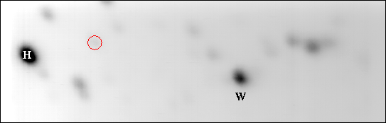The faint star circled in the average image was used as a reference for selecting and re-centring the short exposures. Stars H and W with magnitudes of $I=11.6$ and $I=12.5$ from Cohen et al. (1997) have been labelled in the image. In order to assess the improvement in the performance of the Strehl selection and re-centring obtained by Fourier filtering the short exposures using the diffraction-limited transfer function shown in Figure 5.6, analysis of this dataset was repeated a number of times both with and without the filtering process. Figure 5.10a shows the image obtained when the Strehl ratio and position of the brightest speckle is calculated from the brightest pixel in the image of this star in the sinc-resampled short exposures (with no filtering applied). The exposures with the highest $1\%$ of Strehl ratios were selected and re-centred to produce the image shown in the figure. The sharpness of the point source found at the location of the reference star is artificial - it results from the coherent addition of noise in the original short exposures brought about by the selection and re-centring process as discussed in Chapter 5.4. The images of the other stars in the field are clearly more compact than in the average image of Figure 5.9, indicating that the re-centring process is performing well.

Figure 5.10: Four images of M13 generated using the same $3000$ frames. The reference star used for image selection and re-centring is circled in Figure 5.9. For panel a) the short exposures were not filtered to suppress the noise before the Strehl ratio and position of the brightest speckle were calculated in the reference star image. The best $1\%$ of exposures were selected to produce the image. Panel b) shows the result when the filter described in Figure 5.6 is used to suppress the noise before calculating the Strehl ratio and position of the brightest speckle for the reference star. The best $1\%$ of exposures were selected. Panel c) shows the result of re-centring and co-adding all the exposures without the filtering. Panel d) shows the result when the filtering is used. The typical FWHM for stars on the left-hand side of these images are: a) $300\times 200$ $mas$; b) $280\times 180$ $mas$; c) $400\times 280$ $mas$; and d) $300\times 260$ $mas$.

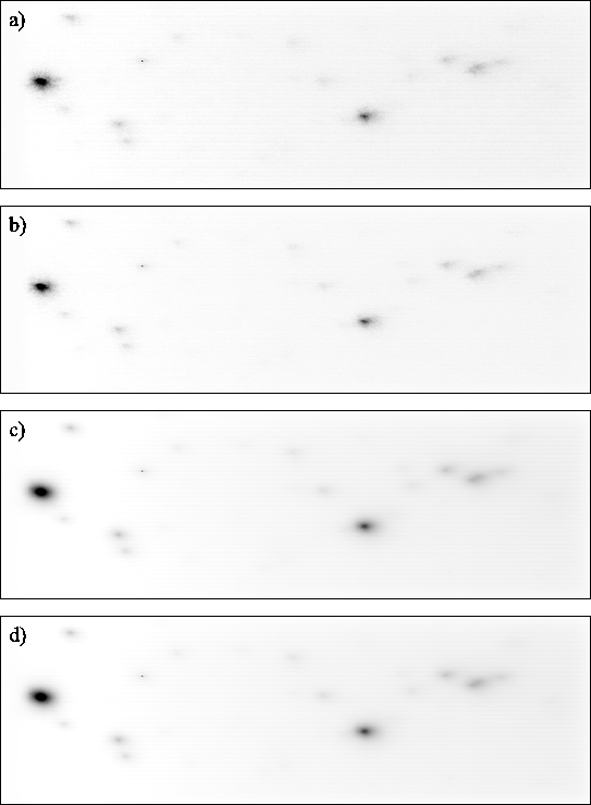Figure 5.10b shows the image obtained when the short exposure images are filtered using the function described in Figure 5.6 before the Strehl ratio and location of the brightest speckle are calculated. The original raw exposures were selected and re-centred based on this data in the same way as for Figure 5.10a. The general characteristics of the image are similar to Figure 5.10a, and the reference star is again artificially sharp. The other stars in the field are slightly more compact in Figure 5.10b with a smaller halo surrounding them. It is clear that the filtering process has improved the image quality.

Figures 5.10c and 5.10d show the results without filtering and with filtering respectively, using all of the short exposures in the run. The smoothness of the halos around the stars makes the improvement in image quality provided by the filtering less apparent for the comparison of these two images than for the case of the selected exposures. The FWHM of stars towards the left-hand side of the field is reduced from $400\times 280$ $mas$ without filtering to $300\times 260$ $mas$ with the filtering, however.

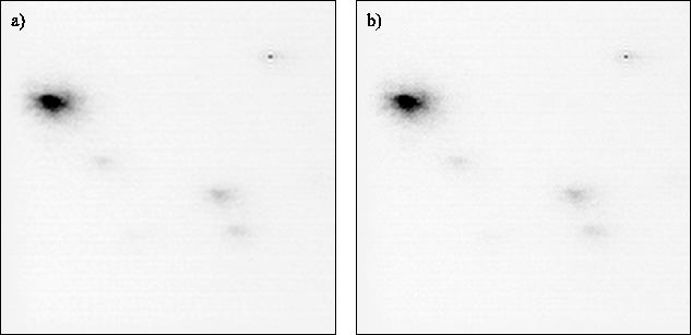
In order to test the performance of the second application of Fourier filtering (the application of the noise filter shown in Figure 5.7 to the selected exposures) I repeated the analysis of Figure 5.10b without filtering the selected exposures when they were re-centred and co-added. The effect of the noise filtering on the final image quality is shown Figure 5.11. This shows an enlargement of part of Figure 5.10b around the left-hand bright star in panel a) using the noise filter, and the result of the same analysis performed without using the noise filter on the selected exposures in b). There is no evidence for blurring of the filtered image, and the highest spatial frequency components in the noise have been suppressed in comparison with Figure 5.11b.

Figure 5.11: Panel a) shows the region of Figure 5.10b around the left-hand bright star. In producing this image the final selected exposures were Fourier filtered in order to suppress noise. Panel b) shows the image obtained without the noise filtering.

The results of the two approaches to Fourier filtering appeared successful, so these filtering procedures were used in the data reduction presented in the remainder of this chapter (except where specifically stated otherwise in the text).