Next: Performance of the Fourier Up: Data reduction Previous: Data reduction Contents
The readout noise from the analogue camera electronics is distributed at a range of spatial frequencies within the images. A significant fraction of this noise appears at spatial frequencies beyond the telescope diffraction limit, and this component of the readout noise is also reduced if high spatial frequencies are suppressed.
There are two clear applications for Fourier filtering in my approach
to the data reduction, as listed in Table 5.6.
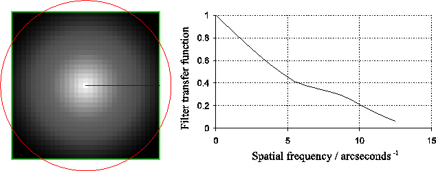
In the first application we want to find bright speckles in the noisy short exposure images. A very effective approach is to search for the peak cross-correlation between the short exposure image and a diffraction-limited telescope PSF. This cross-correlation process is equivalent to multiplying the images by the modulation transfer function of the diffraction-limited telescope in the Fourier domain (effectively convolving the image with a diffraction-limited telescope PSF). In order to minimise the additional computation required, this was implemented during the sinc-resampling process, which is also performed in the Fourier domain. The model for the modulation transfer function which I used was calculated from the autocorrelation of the simple model of the NOT aperture described by Figure 3.4, and I have included a graphical description of the transfer function in Figure 5.6. I used the same geometrical approach for calculating this function as was used for the autocorrelation of two circles in Appendix A (see Equation A.15).
 |
After the filtering and resampling have been completed, the peak in the resampled image corresponds to the most likely location of the brightest speckle. The height of the peak provides a measure of the flux in the brightest speckle, and hence the Strehl ratio. The measured Strehl ratio and position would then be used to select and re-centre the sinc-resampled (but unfiltered) exposures. In the high signal-to-noise regime the peak flux in the filtered short exposures was related to the peak flux in the original exposure by a non-linear, monotonically increasing function. The non-linearity of this function does not introduce complications, however, as the measurements made on the filtered images are simply used to sort the exposures according to their quality, and then to re-centre the selected exposures. Strehl ratios quoted in the text are based on measurements of the brightest pixel in the final Lucky Exposures image.
In the second application of filtering described in
Table 5.6, only spatial Fourier components beyond
![]() can be suppressed without blurring the
astronomical image. However, the dynamic range of sinc-resampled
images is limited by Gibb's phenomena, which can be suppressed only if
the spatial Fourier components of the image are smoothly reduced to
zero below the Nyquist cutoff spatial frequency of the CCD pixel
array. A two dimensional Fourier filter was developed based on the
Hanning window which attempted to suppress both the noise and Gibb's
phenomena whilst minimising the blurring of the image. The filter
function was flat-topped but dropped smoothly to zero before reaching
the Nyquist frequency in all orientations, and also dropped smoothly
to zero at spatial frequencies beyond
can be suppressed without blurring the
astronomical image. However, the dynamic range of sinc-resampled
images is limited by Gibb's phenomena, which can be suppressed only if
the spatial Fourier components of the image are smoothly reduced to
zero below the Nyquist cutoff spatial frequency of the CCD pixel
array. A two dimensional Fourier filter was developed based on the
Hanning window which attempted to suppress both the noise and Gibb's
phenomena whilst minimising the blurring of the image. The filter
function was flat-topped but dropped smoothly to zero before reaching
the Nyquist frequency in all orientations, and also dropped smoothly
to zero at spatial frequencies beyond
![]() in
orientations where
in
orientations where
![]() was lower than the Nyquist
frequency (
was lower than the Nyquist
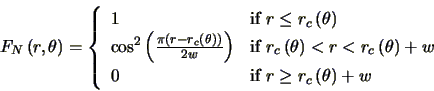
frequency (![]() was taken as the centroid of the observing band). A
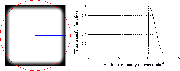
greyscale representation of the filter and cross-section are shown in
Figure 5.7. The value of this filter function
was taken as the centroid of the observing band). A
greyscale representation of the filter and cross-section are shown in
Figure 5.7. The value of this filter function ![]() can be defined in polar coordinates as follows:
can be defined in polar coordinates as follows:
 |
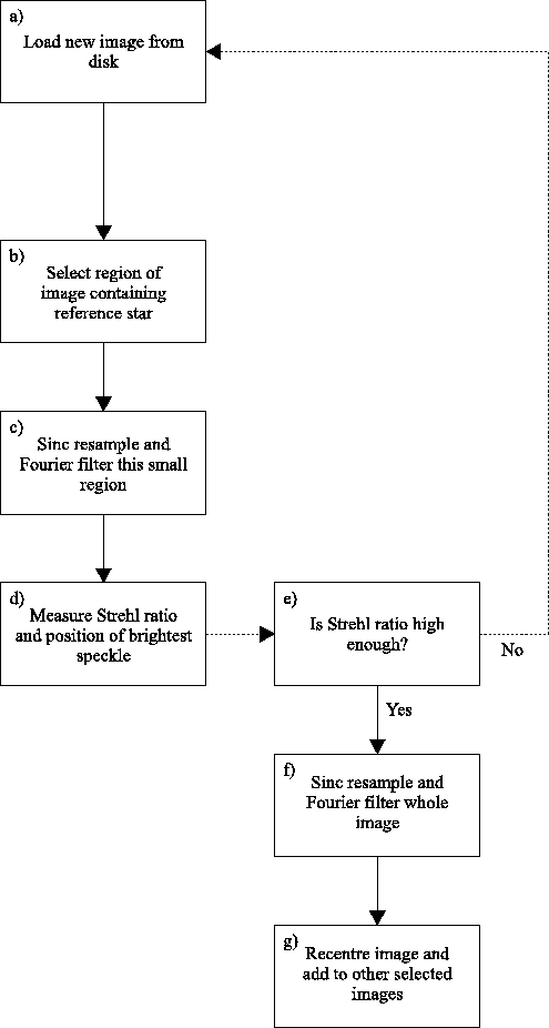
The two applications of spatial filtering mentioned above were incorporated into my approach to the data reduction relatively straightforwardly. In both applications the filtering was implemented in the Fourier domain at the same time as the sinc-resampling of the relevant images. A modified version of the data reduction flow chart of Figure 3.13 incorporating the filtering is shown in Figure 5.8.
Bob Tubbs 2003-11-14