cjo25
Summary and figures of the currently available experimental data on CMB temperature anisotropies. A couple of packages for download, including a C version of the WMAP likelihood code.
NEWS
previous news
- 10.07.03: I am now in Switzerland. News and features on this page.
- 01.07.03: New 'Talks and posters' page here with abstracts and downloads of slides and posters in PDF format.
- 01.07.03: I have come back from Wales and I have put the slides of my seminar here. I am on my way to Switzeland to write up and any other plans can be found here.
- 28.05.03: Less cluttered navigation. Publications now available here. Also, I have added an online research proposal here.
- 16.05.03: Another update, another design :). I have now written my WMAP page with a C version of the likelihood code for download and some recent results.
List of publications with abstracts and links.
List of talks an posters with abstracts and downloads.
|
|
Constraining the shape of the CMB: a Peak-by-peak analysis
Carolina J. Ödman, Alessandro Melchiorri, Michael P. Hobson and Anthony N. Lasenby
The recent measurements of the power spectrum of Cosmic Microwave Background anisotropies are consistent with the simplest inflationary scenario
and big bang nucleosynthesis constraints. However, these results rely on the assumption of a class of models based on primordial adiabatic perturbations, cold dark matter and a cosmological constant. In this paper we investigate the need for deviations from the Λ-CDM scenario by first characterizing the spectrum using a phenomenological function in a 15 dimensional parameter space.
Using a Monte Carlo Markov chain approach to Bayesian inference and a low curvature model template we then check for the presence of new physics and/or systematics in the CMB data. We find that low frequency CMB data tend to predict strong peaks, whereas high frequency data predict a flatter spectrum. Overall, we find an almost perfect consistency between the phenomenological fits and the standard Λ-CDM models. The improved spectral resolution expected from future satellite experiments is warranted for a definitive test of the scenario.
Introduction
The recent observations of the cosmic microwave background (CMB) anisotropies power spectrum have presented cosmologists with the possibility of studying the large scale properties of our universe with unprecedented precision. As is well known, the structure of the theoretical CMB spectrum, given mainly by the relative positions and amplitude of the so-called acoustic peaks, is sensitive
to several cosmological parameters. The existing CMB data sets are therefore being analyzed with increasing sophistication in an attempt to measure the undetermined cosmological quantities.
The recent analyses of this kind have revealed an outstanding agreement between the data and the inflationary predictions of a flat universe and of a primordial scale invariant spectrum of adiabatic density perturbations.
However, the CMB result relies on the assumption of a particular class of models, based on adiabatic, passive and coherent primordial fluctuations, and cold dark matter.
In the present work we check to what extent modifications to the standard Λ-CDM scenario are needed by current CMB observations with two complementary approaches:
First, we provide a model-independent analysis by fitting the data with a phenomenological function and characterizing the observed multiple peaks.
We then compare the position, relative amplitude and width of the peaks with the same features expected in a 4-parameters model template of Λ-CDM spectra.
By doing a peak-by-peak comparison between the theory and the phenomenological fit which is based on a much wider set of parameters, we then verify in a systematic way the agreement with the standard theoretical expectations.
Method
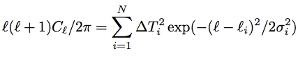
We use a sum of 5 gaussians parametrised by their amplitude, center position and width to generate a phenomenological power spectrum
We then characterize the 15 parameters of our gaussians by fitting the phenomenological power spectra to 3 CMB data combinations: Low frequency experiments, High frequency experiments, and both together. The fitting is performed through an MCMC algorithm (a page on MCMC is under construction. For more details, see Lewis & Bridle, Phys.Rev. D66 (2002)). The table below lists the experimental data used in this study.
| Experiment |
l-range |
reference |
| Low Frequency experiments |
|
|
| DASI |
117 - 836 |
Halverson & al, Ap. J, 568, 38, 2002 |
| CBI |
400 - 1450 |
Pearson & al, 2002 |
| VSAE |
160 - 1400 |
Grainge & al, 2002 |
| High Frequency experiments |
|
|
| Acbar |
150 - 3000 |
Kuo & al, 2002 |
| Archeops |
15 - 350 |
Benoit & al, 2002 |
| Boomerang |
50 - 1000 |
Ruhl & al, 2002 |
| Maxima |
73 - 1161 |
Lee & al, 2001, Ap. J. 561, 2001 |
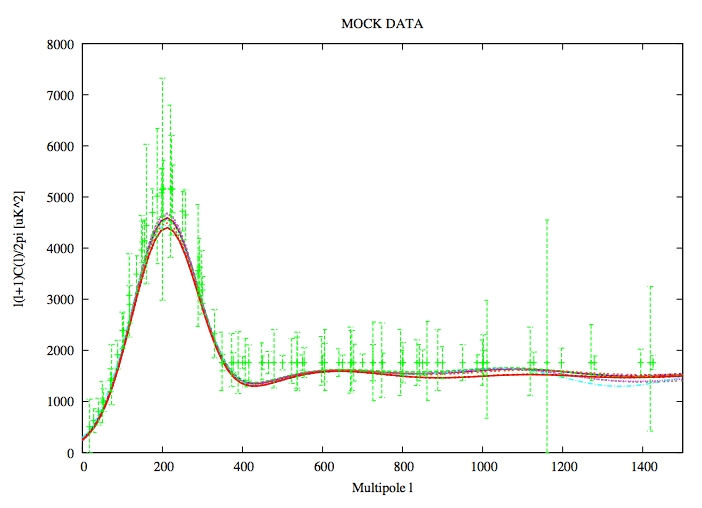
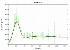
Is a sum of gaussians biased towards the presence of peaks?
In order to test this, we generated a set of mock data by convolving a 'flat' power spectrum with the experimental window functions. Our mock power spectrum consists of a first peak followed by a flat line of constant power. Below are the 10 best-fit samples from out MCMC algorithm. This shows that the gaussians method, with wide priors, is able to fit a flat line. We therefore expect any detection of wiggles to be significant.
(click thumbnail for a bigger image)
Fitting the CMB data with a phenomenological power spectrum
After checking the reliability of our phenomenological function, we proceeded to fit the CMB data as listed in the table above. First, high and low frequency experiments on their own, then together. We used the available window functions and correlation for the band-powers when available. We marginalised analytically over beam and calibration uncertainty, as described in Bridle & al, MNRAS 335, 1193 (2002). When available, we used the lognormal approximation to the band-power (see Bond, Jaffe & Knox, Astrophys.J. 533 (2000) 19, or Knox's Radpack web-page).
We ran our MCMC code to get about 7000 samples for each subset of data. The numbr density of output samples of an MCMC routine is proportional to the joint posterior distribution of the parameters being investigated. We counted our samples into bins and normalised the resulting histograms to get a likelihood function for each parameter.
Below is a table of our results. For each parameter, we show the best-fit marginalised value and 1-σ error.
| Variable | Full data set | High Frequency
data | Low Frequency
data |
| Δ T1 | 69.3-2.3+2.4µ K | 70.7-3.5+4.8µ K | 68.9-4.1+5.5µ K |
| Δ T2 | 44.0-1.9+1.7µ K | 43.1-3.0+3.6µ K | 46.8-4.3+3.6µ K |
| Δ T3 | 43.8-4.4+2.1µ K | 40.7-5.0+4.3µ K | 54.4-11.2+3.4µ K |
| Δ T4 | 31.2-8.7+5.7µ K | 25.7-5.7+3.1µ K | 27.9-7.3+8.7µ K |
| Δ T5 | 19.8-3.8+1.8µ K | 18.4-5.2+3.2µ K | 20.6-17.3+12.7µ K |
| l1 | 208.8-6.1+6.2 | 204.6-7.9+11.4 | 206.8-22.0+10.8 |
| l2 | 550-45+13 | 505-21+25 | 533-20+25 |
| l3 | 824-41+12 | 764-42+74 | 806-36+26 |
| l4 | 1145-45+30 | 1158-67+242 | 1189-87+32 |
| l5 | 1474-79+153 | 1649-262+142 | 1515-346+81 |
| σ1 | 93.3-5.2+4.5 | 90.3-6.2+8.2 | 88.2-12.3+12.7 |
| σ2 | 111.2-27.4+27.7 | 78.2-12.2+19.3 | 61.9unbounded+36.7 |
| σ3 | 82.5-23.1+20.7 | 136.3unbounded+94.2 | 69.8unbounded+12.8 |
| σ4 | not constrained | not constrained | not constrained |
| σ5 | not constrained | not constrained | not constrained |
How well is the power spectrum constrained?
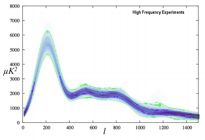
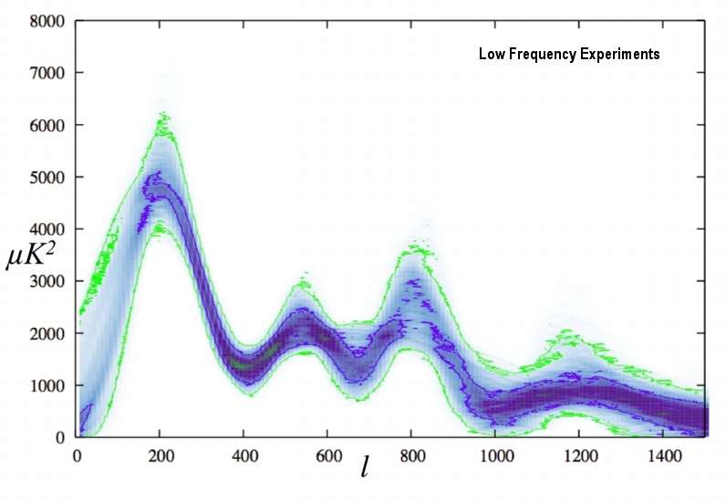
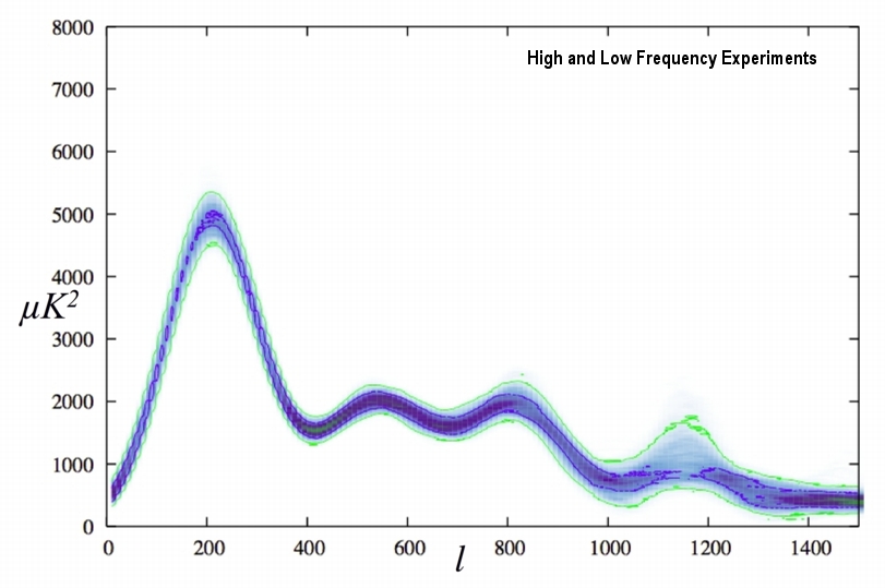
In order to see how well the power spectrum is constrained by the data, provided it is a continuous function with few limits on its shape as our wide priors allow, we proceeded as follows: The power - angular-scale space was divided into pixels. For each MCMC sample, a unit was added in each pixel it went through. This is equivalent to plotting a two-dimensional density plot of our samples in power - angular-scale space. The resulting plots are shown below.
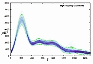 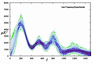 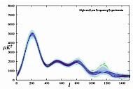
(click thumbnail for a bigger image)
These plots show what the whole spectrum is likely to look like. Certain ranges of angular scale are not within any 1-σ contour. This means either that the data is insufficient, or that it is inconsistent.
We can see from this analysis that low frequency experiments have a tendency to enhance the expected acoustic peaks, whereas the high frequency experiments have a tendency to flatten it. This translates into low-frequency data favouring a higher amount of baryonic matter and a lower spectral index for the initial power spectrum of adiabatic perturbations as explained below.
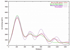
(click thumbnail for a bigger image)
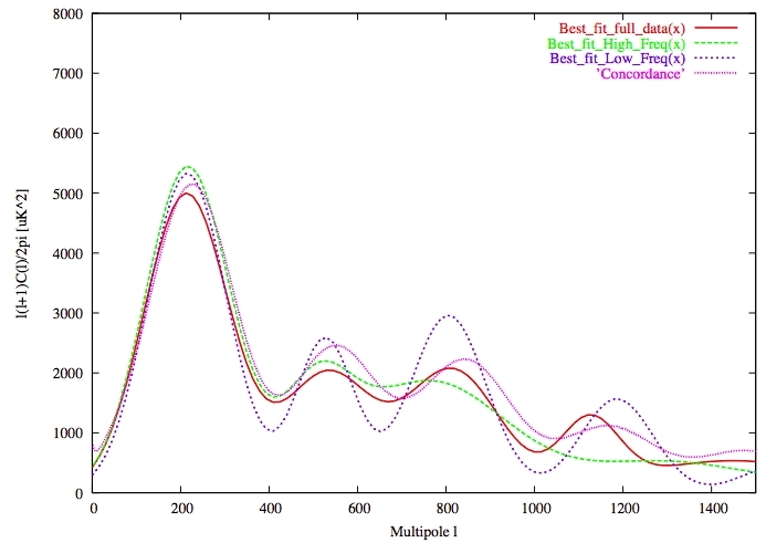
Above is a comparison of the best-fit gaussians for the three data sets and the so-called concordance power spectrum generated using CMBFast. This confirms the higher constrast of the acoustic peaks that seems to arise from the low frequency data. One plausible explanation for the difference between the low and high frequency experiments is that the sources of experimental error are different, as is their treatment. Nevertheless, both results are consistent. In particular, they all detect the expected damping of the power at high multipoles. The best-fit power spectrum obtained by combining both sets of data is very close to the cosmologically-motivated 'concordance model' (Ωm = 0.3, ΩΛ = 0.7).
Relating features to cosmological parameters
In order to relate the phenomenological power spectrum to cosmological parameters, we proceeded to look at a set of CMB observables whose dependence on cosmological parameters is well known. To do so, we considered a database of flat CMB power spectra sampling the various cosmological parameters as follows:
- ωCDM = 0.01, 0.02, ..., 0.40
- ωb = 0.001, 0.002, ..., 0.040
- ΩΛ = 0.0, 0.05, ..., 0.95
- ns = 0.60, 0.62, ..., 1.40
We also use addtional priors:
Weak priors: 0.05 < ΩCDM < 0.5 , 0.15 < Ωbh2 < 0.25 , 0.55 < h < 0.88 , 0.80 < nS < 1.10
Strong priors: 0.10 < ΩCD < 0.35 , 0.18 < Ωbh2 < 0.22 , 0.65 < h < 0.80 , 0.95 < nS < 1.05
For those spectra, we worked out the corresponding Δ Ti, li and &sigmai. We found that spectrum in our database can be fitted better than 10% by the sum of gaussians.
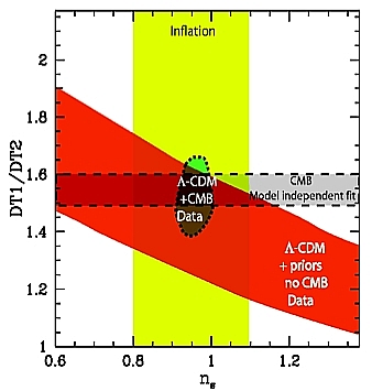
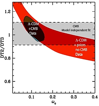
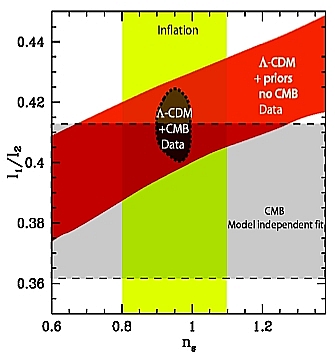
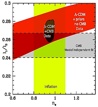
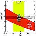
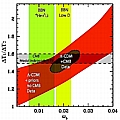
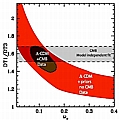
We consider the relative positions and amplitudes of the gaussians, as they are directly related to observable features of the power spectrum. In the following plots, the red region corresponds to the ranges allowed in our database of models. The dark region in the middle shows the region allowed by performing a parameter estimation on our theoretical models. We include other constraints, as described in the figures, and in the paper.
First, a decrease with the initial spectral index decreases the amplitude of the secondary peaks, but that can be compensated by an increase of the optical depth to reionization (τc) which has the effect of dampling the power at small angular scale.
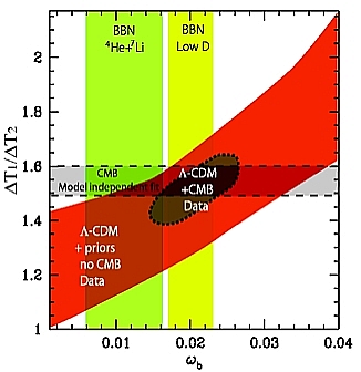
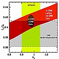
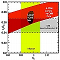
Also, increasing the physical density of baryons (ωb) has the effect of increasing the odd-numbered peaks relatively to the even-numbered ones.
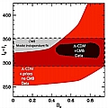
Below are two plots relating the relative amplitudes of the first to the second peak to the spectral index and the density of baronic matter. We also included constraints from inflation regading the spectral index, and from BBN regarding the density of baryons.
(click thumbnail for a bigger image)
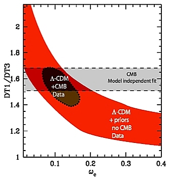
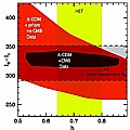
Increasing the density of cold dark matter enhances the third peak. Below, we plot the ratios of the amplitudes of the first to the third and of the second to the third peak vs the physical density of CDM.

(click thumbnail for a bigger image)
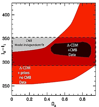
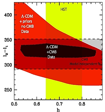
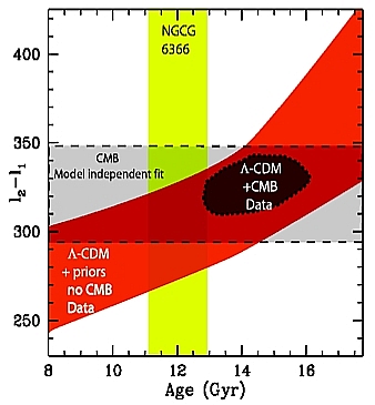
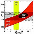
For flat models, changing ΩΛ produces a shift in the position of the peaks as follows (see Melchiorri & Griffiths, New Astronomy Reviews, 45, 2001). It can be characterised by a shift parameter such that l -> Rl, and:
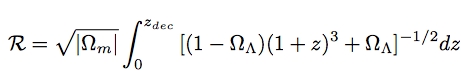
A change in the value of the Hubble parameter produces a similar shift. These two parameters are linked through the age of the Universe by:
Hence, constraints on the relative positions of the peaks should yield constraints on those three parameters. Below, we plot the corresponding observables (positions of the second peaks with respect to the first one) vs those three parameters.
(click thumbnail for a bigger image)
Finally, changing the spectral index also produces a shift, but scale-dependent. Below, we plot the relative positions of the peaks vs nS.
(click thumbnail for a bigger image)
Conclusion
The results obtained here show no need for modifications to the standard model, like gravity waves, quintessence, isocurvature modes, or extra-backgrounds of relativistic particles. Furthermore, possible systematic effects due to unknown foregrounds or calibration and beam uncertainties are not immediately suggested, since the different data sets are consistent with the theory.
In our phenomenological analysis, we found that a straight line (i.e. a flat spectrum) is still 2-σ consistent with the data between 430 < l < 910, but beyond that, the newest experimental results show a damping of the power.
Within the models considered in our database we found (at 68% c.l.): nS = 0.96 ± 0.03, &omegab = 0.022 ± 0.003, ωcdm = 0.12 ± 0.03, ΩΛ = 0.63 ± 0.16, and t0 = 14.2 ± 0.7 Gyrs.
|
|