Isoplanatic angle for atmospheric simulations

The light from two astronomical objects which are separated on the sky by a small angle will travel on slightly different paths through the Earth's atmosphere, as shown schematically in Figure 2.6. If layers of turbulence exist within the atmosphere, the light from the two objects will travel through slightly different parts of each turbulent layer. For two objects separated by a small angle $\Delta \theta$, the offset $x$ in the position of the light paths as they intersect a layer at a height $h$ is given by:

$$x=h\Delta \theta$$ (2.18)

as demonstrated in Figure 2.6. If the offset $x$ between the paths is sufficiently large, the atmospheric perturbations applied to light from the two astronomical targets will differ. This variation in the atmospheric perturbations with angle is closely analogous to the change in the atmospheric perturbations as time elapses and the atmospheric layers move past the telescope in the wind scatter model described in Chapter 2.3.3. Whereas the motion of the atmospheric layers as a function of time was determined by the wind velocities for the wind-scatter case, the relative motion of the atmospheric layers as a function of angular separation from the reference star is determined by the heights of the layers above the telescope.

Figure 2.6: Schematic showing off-axis observations through an atmosphere with two turbulent layers. The off-axis beam passes through the turbulent layers at a position which is offset by an amount proportional to the height of the layer above the telescope (and indicated by $x_{1}$ and $x_{2}$ in the figure).

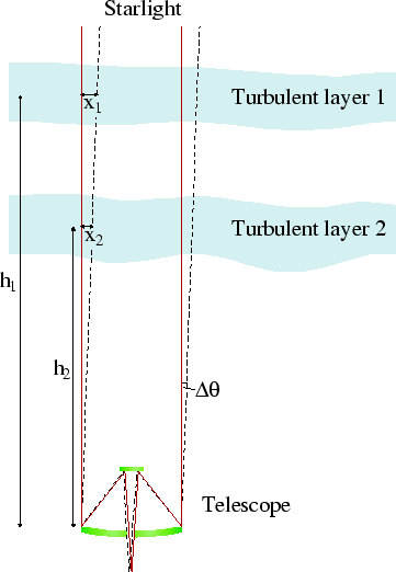The angular separation at which the atmospheric perturbations applied to the light from the two stars becomes uncorrelated is called the isoplanatic angle. For a wind scatter model consisting of thin Taylor screens, the calculation of the isoplanatic angle is undertaken in an identical manner to the calculation of the timescale for decorrelation of the speckle pattern described above. The numerical simulations investigating the effect of relative motions of atmospheric layers on the image plane speckle pattern in Chapter 2.3.3 would be equally applicable to the study of isoplanatic angle, and the results can be used here directly. The similarity between the temporal properties and isoplanatic angle for wind-scatter models has been noted by a number of previous authors including Roddier et al. (1982a).

The calculation of the isoplanatic angle for atmospheres consisting of a number of layers of Kolmogorov turbulence is described in Roddier et al. (1982b), following a similar argument to that for atmospheric coherence time calculations described in Roddier et al. (1982a). The isoplanatic angle is inversely proportional to the weighted scatter $\Delta h$ of the turbulent layer heights:

$$\Delta h=\left [ \frac{ \int h^{2} C_{N}^{2} \left ( h \righ... ...^{2} \left ( h \right ) \mbox{d}h} \right )^{2} \right ]^{1/2}$$ (2.19)

If the atmospheric turbulence is concentrated in a narrow altitude range, then the isoplanatic angle for short exposure imaging will increase with telescope diameter in a fashion exactly analogous to the dependence of the speckle timescale $\tau _{e}$ on telescope diameter for the wind scatter model described in Chapter 2.3.3.

The decorrelation of the speckle pattern for a target with increasing angular distance $\theta$ from a reference star is expected to follow a similar relationship to that for the temporal decorrelation of a speckle pattern (Equation 2.2). The cross-correlation of the speckle patterns $C\left ( \theta \right )$ should thus obey the relationship:

$$C\left ( \theta \right ) = \frac{a^{2}}{a^{2}+\theta^{2}}$$ (2.20)

where $a$ depends on the relative separations of the atmospheric layers.

I have not repeated the numerical simulations here for the case of isoplanatism as the new simulations would be computationally identical to those performed for the measurements of the timescale $\tau _{e}$ - the only difference would be in the units used. The vertical axis in Figure 2.5 is labelled $\tau _{e}$, but it could equally have been labelled isoplanatic angle $\theta_{e}$. The plot would then correspond to the variation in isoplanatic angle as a function of telescope diameter for two models of the atmosphere. The model corresponding to curve A would be an atmosphere with a single layer at an altitude of $h$, with the isoplanatic angle $\theta_{e}$ on the vertical axis plotted in units of $\frac{r_{0}}{h}$ $radians$. The model corresponding to curve B would have two layers each with half the value of $C_{N}^{2}$ and at altitudes of $0.8h$ and $1.2h$.

A number of different measures of the isoplanatic angle have been suggested in the literature. In order to provide consistency with the discussion of atmospheric timescales in Chapters 2.2 and 2.3, I will take the isoplanatic angle $\theta_{e}$ for speckle imaging to be that at which the correlation of the speckle pattern for two objects drops to $\frac{1}{e}$ of the value obtained near the reference star. For an atmosphere consisting of Taylor screens, the value of $\theta_{e}$ will be dependent on the relative motions of the Taylor screens with angle in same way as $\tau _{e}$ depends on the relative motions with time. For the model described by Equation 2.20, $\theta_{e}$ will be:

$$\theta_{e}=\left ( \sqrt{e-1} \right )a$$ (2.21)

Vernin & Muñoz-Tuñón (1994) suggest the isoplanatic angle for short exposure imaging with the full aperture of the NOT will be significantly larger than the isoplanatic angle expected for non-conjugate adaptive optics (or for interferometric techniques involving small apertures). This is due to the turbulent layers being distributed over a narrow range of heights above the telescope. With non-conjugate adaptive optics the isoplanatic angle is determined by the typical height of the turbulence (whereas with large telescope apertures the isoplanatic angle for speckle imaging techniques such as Lucky Exposures is related to the scatter of different altitudes $\Delta h$ over which the turbulence is distributed rather than the absolute height). In calculating the isoplanatic angle for non-conjugate adaptive optics, the deformable mirror (typically positioned in a re-imaged pupil plane) can be treated like an additional layer of atmospheric turbulence which cancels out the phase perturbations along one line of sight, but contributes additional perturbation for objects significantly off-axis.

Measurements of the isoplanatic angle for speckle imaging at a number of observatories have typical given values in the range $1.5$ $as$ to $5$ $as$ for observations at $500$ $nm$ wavelength (see e.g. Vernin & Muñoz-Tuñón (1994); Roddier et al. (1982a)). The isoplanatic angle for speckle observations is expected to be about $70\%$ larger than that for adaptive optics, based on measurements by Vernin & Muñoz-Tuñón (1994). The isoplanatic angle for observations at I-band should be a further factor of two larger due to the relationship between the coherence length $r_{0}$ and the wavelength (Equation 2.9).