Numerical simulations

A number of numerical simulations were undertaken to investigate the temporal properties of Taylor screen models more rigorously. Initially, two models were investigated, the first with a single Taylor screen moving at a constant wind speed as discussed in Chapter 2.3.2, the second having two equal Taylor screens with slightly different wind speeds but the same wind direction. The properties of the two models are summarised in Table 2.1. The Taylor phase screens used had Kolmogorov turbulence extending to an outer scale of $683r_{0}$, with no power on spatial frequencies larger than this. The size of the outer scale was determined by the available computer memory. Both simulations produced wavefront perturbations with the same coherence length $r_{0}$. Images from filled circular apertures with diameters between $3r_{0}$ and $10r_{0}$ were generated at a large number of discrete time points.

Table 2.1: A brief summary of the two model atmospheres investigated. The third column shows the scatter in the wind velocities calculated using Equation 2.10.

Model	Layer velocities	$\Delta v$
1	Single layer of turbulence moving at a speed of $0.15r_{0}$ per timestep	$0$
2	Two layers with equal turbulent strength, moving at $0.12r_{0}$ per timestep and $0.18r_{0}$ per timestep respectively	$0.03r_{0}$ per timestep

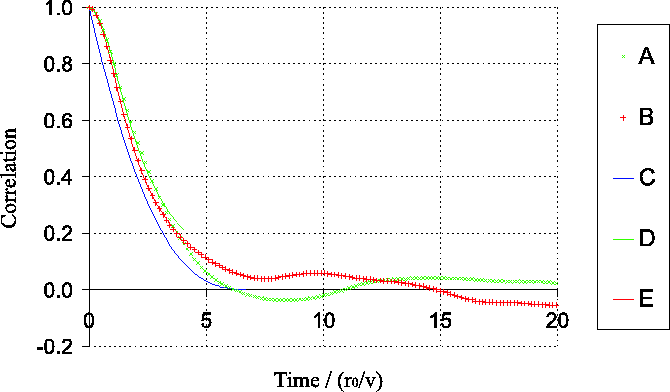
Photometric measurements were made at a fixed point in the image plane corresponding to each of the simulated apertures at each time point, and the temporal autocorrelation of this data was calculated. Figure 2.4 shows two example autocorrelations for an aperture diameter of $7r_{0}$. There is relatively good agreement between the model of Aime et al. (1986) (Equation 2.2) and the normalised autocorrelation data from numerical simulations up to time differences corresponding to the coherence timescale $\tau _{e}$. For larger time differences Equation 2.2 tends quickly to zero, while the simulation data usually drifted either side of zero somewhat. This may be due to the limited timescale of the simulations (a few hundred times $\tau _{e}$, which is not long enough to average very many realisations of the longer timescale changes in the speckle pattern). Similar results were found for all of the aperture diameters simulated, and the temporal power spectra were found to agree with the model of Aime et al. (1986).

Figure 2.4: Two examples of the temporal autocorrelation curves generated from numerical simulations (and used to produce Figure 2.5). The curves have been normalised using the method described in Chapter 2.2.1. A shows the result for a single layer atmosphere and B for a two-layer atmosphere (models 1 and 2 from Table 2.1 respectively). C shows the predicted decorrelation using the highly simplified model for a single layer atmosphere described in Appendix A. D and E show least-squared fits of the form of Equation 2.2 to the early parts of curves A and B respectively.

The coherence timescale $\tau _{e}$ was then calculated from each simulation using the method described in Chapter 2.2.1. A plot of the variation of the coherence timescale with telescope aperture diameter is shown in Figure 2.5.

Figure 2.5: Timescale $\tau _{e}$ for a range of aperture diameters, for the two atmospheric models. Curve A shows the result for a single Taylor screen of frozen Kolmogorov turbulence. B is a similar plot for the two layer atmosphere listed as model 2 in Table 2.1. The error bars simply indicate the standard error of the mean calculated from the scatter in results from a number of repeated Monte Carlo simulations. Errors in the measurements at different aperture diameters are partially correlated as the same realisations of the model atmospheres were used for all the aperture diameters shown. The red line is described by Equation 2.14 and the black horizontal line is at the value given in Equation 2.15.

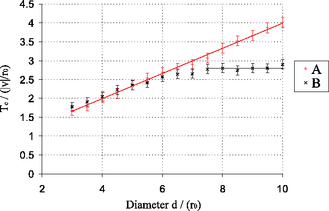The red line in Figure 2.5 is a linear regression fit to the measured timescale $\tau _{e}$ for simulations with a single Taylor screen. The equation for this best fit line is:

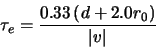$$\tau_{e} = \frac{0.33\left (d+2.0 r_{0}\right )}{\left \vert v \right \vert }$$ (2.14)

The timescale appears to depend approximately linearly on the aperture diameter $d$, as predicted in Appendix A. The value of $\tau _{e}$ was found to be larger than predicted by my simplified model by a constant amount $\sim 2r_{0}/\left \vert \mathbf{v} \right \vert$. This is consistent with a small region of the atmospheric layers extending $\sim r_{0}$ into areas $A$ and $C$ in Figure A.3 being correlated with the phase perturbations in area $B$. The same hypothesis would explain why the measured temporal autocorrelations shown in Figure 2.4 as curves A and B lie to the right of the prediction corresponding to my simplified model (curve C) over the left-hand part of the graph.

For small aperture diameters, the simulations with a two-layer atmosphere have very similar timescales to those with a single atmospheric layer. However there is a knee at $D\simeq 6r_{0}$, and at diameters larger than this the timescale $\tau _{e}$ appears to be constant at:

$$\tau_{e} \sim 2.8\frac{r_{0}}{\left \vert v\right \vert}$$ (2.15)

where $\left \vert v\right \vert$ is the average wind velocity for the two layers. It is of interest to compare this timescale with that predicted by Equations 2.11 and 2.12. For this atmospheric model, the wind scatter $\Delta v$ is equal to:

$$\Delta v = 0.2 \left \vert v \right \vert$$ (2.16)

The timescale $\tau _{e}$ can be written in terms of $\Delta v$:

$$\tau_{e} \sim 0.56\frac{r_{0}}{\Delta v}$$ (2.17)

This is larger than the timescales predicted by both Equation 2.11 (from Roddier et al. (1982a)) and Equation 2.12 (from Aime et al. (1986)). The result of Aime et al. (1986) is within $3\sigma$ of these simulations however (remembering that the errors in the simulations are correlated for different aperture diameters).

Figure 2.5 implies that the timescale for changes in the speckle pattern found at the focus of a well figured astronomical telescope may increase somewhat with aperture diameter if the atmospheric turbulence is moving with a common wind velocity. This would not be the case if there is a substantial scatter in the wind velocities, as the timescale saturates at a level close to that predicted by Equation 2.12. Vernin & Muñoz-Tuñón (1994) found that the scatter in the velocities of the turbulent layers above the NOT is small enough that the timescale for speckle patterns using the full aperture of the NOT should be twice the timescale which would be found with small apertures, or that for standard adaptive optics correction. This is consistent with measurements by Saint-Jacques & Baldwin (2000) which indicated that a single wind velocity (or narrow range of wind velocities) dominates above La Palma. This contrasts with results at a number of other observatories (e.g. Parry et al. (1979); Vernin & Roddier (1973); Caccia et al. (1987); Roddier et al. (1993)) where either strong turbulence is found in several layers with differing wind velocities, or there is little evidence for any bulk motion of the atmospheric perturbations across the telescope aperture. Wilson (2003) also found evidence for significant dispersion in the wind velocities above the WHT on some nights.