Timescale measurements for atmospheric simulations

In this section I will develop a number of models for the effect of the Earth's atmosphere on astronomical observations. Refractive index fluctuations in the Earth's atmosphere will be included in a number of thin horizontal layers in the model atmospheres. These layers will remain unchanged, but will move at a constant horizontal velocity intended to represent the local wind velocity, as shown schematically in Figure 2.3. Most previous authors (e.g. Conan et al. (1995)) have also assumed that the structure of these layers remains unchanged as they are blown past the telescope by the wind. This assumption is based upon the work of Taylor (1938) which argues that if the turbulent velocity within eddies in a turbulent layer is much lower than the bulk wind velocity then one can assume that the changes at a fixed point in space are dominated by the bulk motion of the layer past that point. The wind-blown, unchanging turbulent layers used for simulations are often called Taylor phase screens. It should perhaps be noted that Taylor's original argument applied to atmospheric measurements at a single fixed point, and may not be strictly true for the case of a telescope with large diameter. The Earth's curvature can be ignored for such simulations, and the perturbing layers are taken to be parallel planes above the ground surface.

The layered model of atmospheric turbulence used for my simulations is supported by a number of experimental studies at Roque de los Muchachos observatory, La Palma (Vernin & Muñoz-Tuñón (1994); Wilson & Saunter (2003); Avila et al. (1997)); the model would also provide realistic results for many other good observatory sites.

Figure 2.3: When turbulent mixing of air with different refractive indices occurs in the atmosphere, phase perturbations are introduced into starlight passing through it. Experimental measurements at a number of astronomical observatories have indicated that these refractive index fluctuations are usually concentrated in a few thin layers in the atmosphere. Two layers are shown in the above figure, each expected to travel at the local wind velocity.

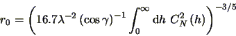
Following the work of Tatarski (1961), the refractive index fluctuations within a given layer in the simulations can be described by their second order structure function:

$$D_{N}\left(\mathbf{\rho} \right) = \left \langle \left \vert... ...{\rho} \right ) \right \vert ^{2} \right \rangle _{\mathbf{r}}$$ (2.4)

where $N \left ( \mathbf{r} \right )$ is the refractive index at position $\mathbf{r}$ and $D_{N} \left ({\mathbf{\rho}} \right )$ is the statistical variance in refractive index between two parts of the wavefront separated by a distance $\mathbf{\rho}$ in an atmospheric layer. For the case of an isotropic turbulent layer following the Kolmogorov model, this structure function $D_{N}$ depends only on the strength of the turbulence:

$$D_{N}\left(\mathbf{\rho} \right) = C_{N}^{2} \left \vert \mathbf{\rho} \right \vert^{2/3}$$ (2.5)

where $C_{N}^{2}$ is simply a constant of proportionality which describes the strength of the turbulence. For the case of an atmosphere stratified into a series of horizontal layers, $C_{N}^{2}\left ( h \right )$ can be taken as a function of the height $h$ above ground level. Under these conditions Equation 2.5 will only be valid within a layer of constant $C_{N}^{2}$.

The phase perturbations introduced into wavefronts by this layered atmosphere can be described by the second order structure function for the phase perturbations (Equation 1.3). This function is dependent on the integral of $C_{N}^{2}\left ( h \right )$ along the light path $z$ and the wavenumber $k$ as follows:

$$D_{\phi_{a}} \left (\mathbf{\rho} \right ) = 2.91k^{2} \left... ...int_{0}^{\infty}\mbox{d}z\mbox{ } C_{N}^{2} \left ( h \right )$$ (2.6)

( $D_{\phi_{a}}\left (\mathbf{\rho} \right )$ here is equivalent to $D_{S}\left(\mathbf{\rho} \right)$ in Tatarski (1961)).

Equation 2.6 can be more conveniently described in terms of wavelength $\lambda$ and the angular distance of the source from the zenith $\gamma$:

$$D_{\phi_{a}} \left (\mathbf{\rho} \right ) = \left ( 115\lam... ...\right ) \right ) \left \vert \mathbf{\rho} \right \vert^{5/3}$$ (2.7)

Using Equations 1.4 and 2.7 we can also write $r_{0}$ in terms of $C_{N}^{2}\left ( h \right )$:

$$r_{0}=\left ( 16.7\lambda^{-2}\left ( \cos \gamma \right )^{... ...y}\mbox{d}h\mbox{ } C_{N}^{2}\left (h \right ) \right )^{-3/5}$$ (2.8)

The amplitude of the refractive index fluctuations described by $C_{N}^{2}\left ( h \right )$ varies only weakly with wavelength $\lambda$ at red and infra-red wavelengths, so the variation of $r_{0}$ with wavelength can be approximated by:

$$r_{0}\propto \lambda^{6/5}$$ (2.9)

For observations in different wavebands, this relationship determines the physical diameter of telescope which would be suitable for the Lucky Exposures method. The work presented in this thesis was carried out between $0.7$ and $1.0$ $\mu m$. Under good seeing conditions, the $7r_{0}$ apertures discussed in Chapter 1.2.3 would correspond to between $2$ and $3$ $m$ diameter telescopes at these wavelengths. For observations in the near infra-red K-band $7r_{0}$ would correspond to $8$ $m$, while at B-band $7r_{0}$ telescopes would have $1$ or $1.5$ $m$ diameter.

Saint-Jacques & Baldwin (2000) undertook detailed atmospheric seeing measurements with the Joint Observatory Seeing Experiment (JOSE - Saint-Jacques et al. (1997); Wilson et al. (1999)) at the William Herschel Telescope, located at the same observatory as the NOT. The experimental setup consisted of an array of Shack-Hartmann sensors capable of measuring the wavefront tilt as a function of position and time in the aperture plane (see Figure 1.9). They found experimentally that the dominant atmospheric phase fluctuations at the William Herschel Telescope (WHT) are frequently associated with a single wind velocity, but also found evidence for gradual change in the phase perturbations applied to wavefronts as the perturbations progressed downwind. This can be explained either by turbulent boiling taking place within an atmospheric layer as it is blown past the telescope, or by the turbulence associated experimentally with one layer actually being distributed in several separate screens, with a narrow range of different wind velocities for the each of the screens (distributed about the measured mean wind velocity). This evolution of the turbulent structure for an atmospheric layer is consistent with the decorrelation with time of turbulent layers found by Caccia et al. (1987), although unlike Roque de los Muchachos observatory they found the typical atmosphere above Haute-Provence to have several such turbulent layers travelling at distinctly different wind velocities. Similar experiments were undertaken using binary stars at the WHT by Wilson (2003). The SLODAR technique (Wilson, 2002) was applied to these binary observations to obtain the heights of the turbulent layers as well as their wind velocities. Preliminary results provided by Wilson (2003) indicated that several turbulent layers with very different wind velocities were present on some of the nights. On at least one night, most of the turbulence was found at very low altitude above the WHT, and it is not necessarily certain that the same conditions would be present at the NOT further up the mountain.

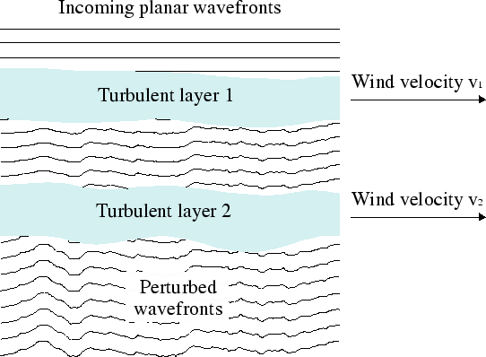
For my numerical simulations I have ignored the possibility of turbulent boiling taking place within individual atmospheric layers because of the lack of a suitable mathematical model for the boiling process. Models which are free of boiling but which have multiple Taylor screens with a scatter of wind velocities describing each individual atmospheric layer can adequately fit existing experimental results, and these are the most widely used models for atmospheric simulations. This form of multiple Taylor screen model is usually known as a wind-scatter model.

Each of the atmospheric layers has a characteristic velocity for bulk motion ($v_{1}$ and $v_{2}$ for the two layers in Figure 2.3) corresponding to the mean local wind velocity at the altitude of the layer.