Next: Resolution and spatial frequency Up: Results with binary stars Previous: Varying the fraction of Contents
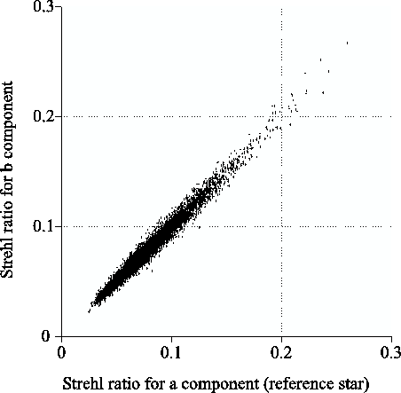 |
Figure 3.22 compares the Strehl ratios of the
brightest speckle in the PSF obtained from each of the stars in
individual exposures. This comparison is not sensitive to variations
in the relative positions of the brightest speckles for the two
stars. In observations of distant ground-based artificial light
sources through a turbulent medium, Englander et al. (1983) found relative
motions in the position of the brightest speckle in Lucky Exposures for light
sources which were separated in the object plane but within the
isoplanatic patch. A qualitative discussion of this effect for
astronomical observations is also found in
Dantowitz et al. (2000); Dantowitz (1998). If such a variation occurs in the
relative positions of the brightest speckles for the two components of
![]() Boötis, this will lead to blurring of the image of the
companion star when the short exposures are re-centred and co-added
based on measurements of the reference star.
Boötis, this will lead to blurring of the image of the
companion star when the short exposures are re-centred and co-added
based on measurements of the reference star.
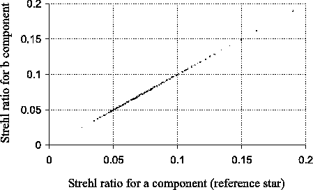
In order to investigate the magnitude of this effect, the short
exposures were sorted by Strehl ratio into groups which each contained
![]() of the total number of exposures. The exposures in each group
were then re-centred and co-added based on the measured positions of
the brightest speckle for the reference star. This gave a single
averaged PSF for the exposures in that group. The Strehl ratios for
binary component b are plotted against the Strehl ratios for the
reference star (component a) in Figure 3.23 for
each of the summed images generated in this way. There is
extremely good correlation between the Strehl ratios for the two
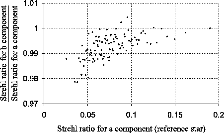
stars, as emphasised by Figure 3.24. In this Figure,
the Strehl ratio for component b has been divided by the Strehl ratio
for component a for each of the summed images. The Strehl ratios for
component b are typically only
of the total number of exposures. The exposures in each group
were then re-centred and co-added based on the measured positions of
the brightest speckle for the reference star. This gave a single
averaged PSF for the exposures in that group. The Strehl ratios for
binary component b are plotted against the Strehl ratios for the
reference star (component a) in Figure 3.23 for
each of the summed images generated in this way. There is
extremely good correlation between the Strehl ratios for the two
stars, as emphasised by Figure 3.24. In this Figure,
the Strehl ratio for component b has been divided by the Strehl ratio
for component a for each of the summed images. The Strehl ratios for
component b are typically only ![]() lower than those for the
reference star although there is a more significant difference for the
poorest exposures. It is clear from these Figures that there must be
very good correlation between the positions of the brightest speckle
for the two stars, and that measurements of the position of the
brightest speckle using a reference star can reliably be used for
re-centring images of another object in the field.
lower than those for the
reference star although there is a more significant difference for the
poorest exposures. It is clear from these Figures that there must be
very good correlation between the positions of the brightest speckle
for the two stars, and that measurements of the position of the
brightest speckle using a reference star can reliably be used for
re-centring images of another object in the field.
 |
 |
The precise shape of the PSF obtained for the reference star and also that for other objects in the vicinity of a reference star is of interest in determining the applicability of the Lucky Exposures method for astronomical programs. The extent of the wings of the PSF determines the area of sky around bright stars which will be ``polluted'' by photon shot noise from starlight. If the image of the reference star is sufficiently similar to the PSF obtained for other objects in the field it can be used for deconvolving the astronomical image. For this reason I undertook an investigation of the faint wings of the PSF, and the differences between the PSF obtained for the reference star and that for the binary companion.
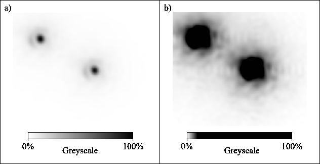
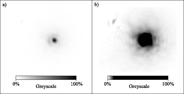
Figure 3.25 shows the best ![]() of exposures of
of exposures of
![]() Boötis using the brighter (left-hand) component as a
reference for Strehl ratio measurements.
Figure 3.25a shows a linear greyscale ranging
from zero to the maximum flux in the image.
Figure 3.25b shows the same image with a
stretched linear greyscale ranging from zero to one-tenth of the
maximum flux. In order to investigate the level of similarity between
the PSFs for the two binary companions, I subtracted the
image of the right-hand star from the image of the left-hand star. A
copy of the image shown in Figure 3.25 was
multiplied by the intensity difference between the two stars, shifted
by the separation of the stars and subtracted from the original
image. This eliminated most of the flux from the left-hand star, as
shown in Figure 3.26. The small residual
component visible in the greyscale-stretched version of this image
shown in Figure 3.26b is largely due to a
small error in the measured separation of the stars due to the finite
pixel size used. There is no clear evidence for anisoplanatism
between the two binary components.
Boötis using the brighter (left-hand) component as a
reference for Strehl ratio measurements.
Figure 3.25a shows a linear greyscale ranging
from zero to the maximum flux in the image.
Figure 3.25b shows the same image with a
stretched linear greyscale ranging from zero to one-tenth of the
maximum flux. In order to investigate the level of similarity between
the PSFs for the two binary companions, I subtracted the
image of the right-hand star from the image of the left-hand star. A
copy of the image shown in Figure 3.25 was
multiplied by the intensity difference between the two stars, shifted
by the separation of the stars and subtracted from the original
image. This eliminated most of the flux from the left-hand star, as
shown in Figure 3.26. The small residual
component visible in the greyscale-stretched version of this image
shown in Figure 3.26b is largely due to a
small error in the measured separation of the stars due to the finite
pixel size used. There is no clear evidence for anisoplanatism
between the two binary components.
 |
The remaining binary component in Figure 3.26 represents a good measure of the PSF for imaging in the vicinity of a reference star using the Lucky Exposures method. The compact image core and steeply decaying wings around the star in this figure indicate that high resolution, high dynamic range imaging will be possible using the Lucky Exposures technique.
 |
The subtracted image in Figure 3.26 allowed
investigation of the faint wings of the PSF for component b without
strong effects from the contribution of the reference star (component
a). Figure 3.27 shows profiles through the image
in Figure 3.26. Curve X in
Figure 3.27a shows a single cross-section along a
line perpendicular to the separation vector between the two stars,
passing through binary component b. Curve Y shows the
flux averaged around the circumference of a circle centred on the
star, plotted as a function of the circle radius (i.e. a radial
profile). At large distances from the core, the flux in the
PSF drops off exponentially in both of these curves (with an
![]() -folding distance of
-folding distance of ![]()
![]() ). This is highlighted in the
logarithmic plots of the same curves shown in
Figure 3.27b. The kink at
). This is highlighted in the
logarithmic plots of the same curves shown in
Figure 3.27b. The kink at ![]()
![]() in the
radial profile plot corresponds to the location of the reference star,
indicating that it was not fully subtracted from the images. For
comparison the profile of a diffraction-limited PSF sampled with the
same pixel scale is shown in both figures as curve Z.
in the
radial profile plot corresponds to the location of the reference star,
indicating that it was not fully subtracted from the images. For
comparison the profile of a diffraction-limited PSF sampled with the
same pixel scale is shown in both figures as curve Z.
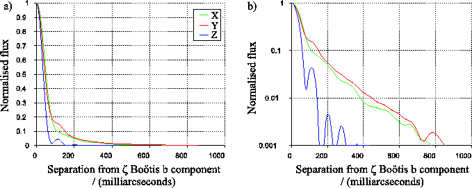 |
If a large number of selected exposures are co-added, the speckle patterns in the wings of the PSF will average out to give a smooth halo. If the flux in this halo follows the exponentially decaying radial distribution shown by curves X and Y of Figure 3.27, then the halo flux could be removed using deconvolution with a simple axisymmetric, exponentially decaying model for the PSF. This would only leave a small residual component from the photon shot noise and small deviations of the PSF halo from the model. It is clear from the rapid decay of the curves in Figure 3.27 that very high dynamic range imaging should be possible, even within relatively crowded fields.