Resolution and spatial frequency response

Both the Lucky Exposures method and the conventional approach of shifting and co-adding all the exposures preserve the Fourier phase information in the images very effectively. For both methods the Fourier amplitudes are reduced (by the modulation transfer function). In order to compare the high resolution imaging performance of the Lucky Exposures and shift-and-add methods, I computed a number of Fourier autocorrelations using some of the data taken on $\zeta$ Boötis, and have displayed them in Figure 3.28. These Fourier autocorrelations preserve the Fourier amplitude information, although all phase information is lost. The Fourier autocorrelation provides a more intuitive representation of the high resolution performance than the modulation transfer function, as the structures in the image autocorrelation can be related directly to structure in the images.

Figure 3.28: Spatial autocorrelations calculated from exposures of $\zeta$ Boötis from the first of the two runs on 2000 May 13. Exposures where the binary components are less than $16$ pixels from edge of the usable region of the CCD have been excluded. a) shows the summed autocorrelation of all the raw exposures; b) shows the summed autocorrelation of the exposures with the highest $1\%$ of Strehl ratios; c) shows the autocorrelation of the shift-and-add image generated from the raw data; and d) shows the autocorrelation of the shift-and-add image of the exposures with the highest $1\%$ of Strehl ratios. The FWHM of these autocorrelations are: a) $0.44$ $as$; b) $0.22$ $as$; c) $0.61$ $as$; and d) $0.24$ $as$.

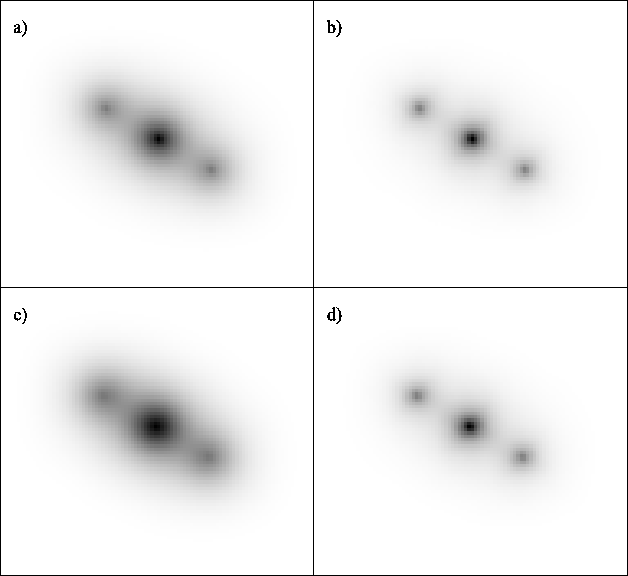Figure 3.28a shows the summation of the autocorrelations for all the short exposures used in the analysis. This image essentially represents the method of Labeyrie (1970) as applied to our data on $\zeta$ Boötis. Figure 3.28b shows the summation of the autocorrelations for only those exposures having the highest $1$% of Strehl ratios. This autocorrelation has a much more compact core and a fainter halo, indicating that the best $1$% of exposures preserve significantly more high spatial frequency information.

It is now of interest to compare the autocorrelations of Figure 3.28a and 3.28b (generated directly from the raw data) with the autocorrelations obtained after the short exposures have been processed using either the conventional shift-and-add approach or using the Lucky Exposures method. Figure 3.28c shows the autocorrelation generated from the conventional shift-and-add image based on the same exposures as were used in Figure 3.28a. The shift-and-add process has produced a substantial reduction in the sharpness of the final autocorrelation, which indicates that the shift-and-add image itself is somewhat degraded in resolution. On the other hand, the autocorrelation of the shift-and-add image generated using the selected exposures (Figure 3.28d) is almost as sharp as that generated directly from the original exposures (Figure 3.28b). It is clear that with the Lucky Exposures method, one benefits not only from the higher resolution of the selected exposures themselves, but also from a substantial improvement in the performance of the shift-and-add process when it is applied to these high Strehl ratio exposures.