Next: Anisoplanatism Up: Results with binary stars Previous: Resolution and spatial frequency Contents
The short exposure images of ![]() Boötis in the first run were
first sorted in order of the Strehl ratio measured on the brighter
component. The exposures were then binned into groups of exposures
with similar Strehl ratios, each group containing
Boötis in the first run were
first sorted in order of the Strehl ratio measured on the brighter
component. The exposures were then binned into groups of exposures
with similar Strehl ratios, each group containing ![]() % of the total
exposures. The exposures in each group were then shifted and co-added,
reducing the dataset to
% of the total
exposures. The exposures in each group were then shifted and co-added,
reducing the dataset to ![]() images, each representing one of the
groups.
images, each representing one of the
groups.
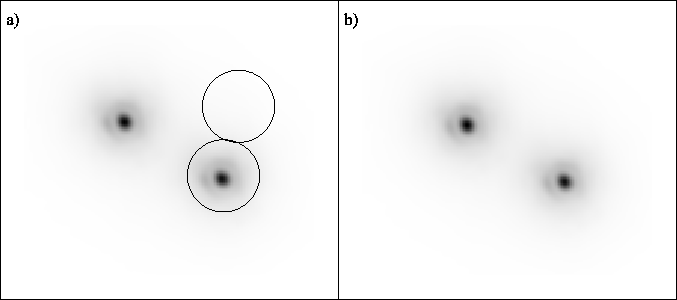
The signal-to-noise measurement described above was applied to these
![]() images using the b component of
images using the b component of ![]() Boötis (the a
component had been used as the reference star). The region around the
b component used for the ``signal'' measurements was limited to the
circle around the star shown in Figure 3.29a. A
circular flat-topped window which dropped smoothly to zero at the
edges (similar to a Hanning window) was used to extract a finite
region of the image data without introducing high frequency noise
components at the boundaries of the circle. A similar section of the
image away from the stars was used for noise measurements (shown by
the upper circle in the image). The range of spatial frequencies used
to represent
high resolution in the image was initially chosen (rather
arbitrarily) as those ranging between
Boötis (the a
component had been used as the reference star). The region around the
b component used for the ``signal'' measurements was limited to the
circle around the star shown in Figure 3.29a. A
circular flat-topped window which dropped smoothly to zero at the
edges (similar to a Hanning window) was used to extract a finite
region of the image data without introducing high frequency noise
components at the boundaries of the circle. A similar section of the
image away from the stars was used for noise measurements (shown by
the upper circle in the image). The range of spatial frequencies used
to represent
high resolution in the image was initially chosen (rather
arbitrarily) as those ranging between ![]()
![]() and
and
![]()
![]() , and the image power spectrum was summed in
two dimensions over these spatial frequencies. The effect of varying
this range of spatial frequencies will be discussed later.
, and the image power spectrum was summed in
two dimensions over these spatial frequencies. The effect of varying
this range of spatial frequencies will be discussed later.
 |
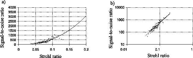
The signal-to-noise ratio ![]() for high spatial frequencies calculated
in this way is plotted against the Strehl ratio
for high spatial frequencies calculated
in this way is plotted against the Strehl ratio ![]() for the
reference star in the images in Figure 3.30a. Also
shown is the best fitting function of the form:
for the
reference star in the images in Figure 3.30a. Also
shown is the best fitting function of the form:
| (3.4) |
 |
Now that we have a relationship between the Strehl ratio of the short
exposures and ![]() , our measure of the signal-to-noise ratio, we can
make a concerted effort to produce the image with the maximum
signal-to-noise ratio using the data on
, our measure of the signal-to-noise ratio, we can
make a concerted effort to produce the image with the maximum
signal-to-noise ratio using the data on ![]() Boötis. If the
individual exposures are treated as independent, uncorrelated
measurements, then the signal-to-noise ratio should be maximised if
all the exposures are selected, but the individual exposures are
weighted according to their Strehl ratios.
Boötis. If the
individual exposures are treated as independent, uncorrelated
measurements, then the signal-to-noise ratio should be maximised if
all the exposures are selected, but the individual exposures are
weighted according to their Strehl ratios.
The data from the first run on ![]() Boötis were processed in this
way, with the individual exposures weighted by a value
Boötis were processed in this
way, with the individual exposures weighted by a value ![]() proportional to our signal-to-noise estimate:
proportional to our signal-to-noise estimate:
| (3.5) |
If the signal-to-noise criteria ![]() used to determine the
signal-to-noise ratio for high resolution imaging is modified, and the
same analysis is followed through, then the Strehl ratio of the final
image from the weighted exposures approach will be different. A number
of different measures of signal-to-noise were tested, either utilising
different ranges of spatial frequencies, or weighted proportionately
with the image Strehl ratio. For all the weighting models tested, I
also generated images with similar Strehl ratios using the simple
exposure selection method without weighting. The images generated
using exposure selection always gave similar signal-to-noise ratios to
the images generated using exposure weighting. With faint reference
stars the accuracy of the Strehl ratio measurements is dependent on
the Strehl ratio itself, and the choice of optimum weighting function
becomes very complex. The complexity of the various weighting models,
their dependence on the numerous aspects of the observations which
affect the accuracy of Strehl ratio measurements, and the increased
computational requirements make this approach less favourable than
simple exposure selection. The analyses in the remainder of this
thesis will be restricted to exposure selection without weighting of
the exposures.
used to determine the
signal-to-noise ratio for high resolution imaging is modified, and the
same analysis is followed through, then the Strehl ratio of the final
image from the weighted exposures approach will be different. A number
of different measures of signal-to-noise were tested, either utilising
different ranges of spatial frequencies, or weighted proportionately
with the image Strehl ratio. For all the weighting models tested, I
also generated images with similar Strehl ratios using the simple
exposure selection method without weighting. The images generated
using exposure selection always gave similar signal-to-noise ratios to
the images generated using exposure weighting. With faint reference
stars the accuracy of the Strehl ratio measurements is dependent on
the Strehl ratio itself, and the choice of optimum weighting function
becomes very complex. The complexity of the various weighting models,
their dependence on the numerous aspects of the observations which
affect the accuracy of Strehl ratio measurements, and the increased
computational requirements make this approach less favourable than
simple exposure selection. The analyses in the remainder of this
thesis will be restricted to exposure selection without weighting of
the exposures.