Anisoplanatism

The isoplanatic angle for the Lucky Exposures technique $\theta_{e}$ should be very similar to the angle at which the speckle patterns for the two stars have decorrelated by a factor of $\frac{1}{e}$ . The argument for this is based on the direct parallels between the decorrelation of the speckle pattern as a function of angle and the decorrelation of the speckle pattern as a function of time discussed in Chapter 2.4. Measurements in Chapter 3.4.3 indicated that the decrease in the Strehl ratio with time followed the decorrelation occurring at another (arbitrary) point in the speckle pattern with time, and the same relationship would be expected as a function of angle between the reference star and an off-axis target. The isoplanatic angle $\theta_{e}$ is thus expected to be analogous to the timescale $\tau _{e}$ for changes in the speckle pattern.

Measurements of $\theta_{e}$ would ideally be obtained from simultaneous observations of a target very close to the reference star, and another target at a separation which produced a Strehl ratio lower by a factor of $\frac{1}{e}$ . As appropriate data is not available here, a model of the effect of atmosphere is required in order to extrapolate the results, leading to some uncertainty in the accuracy of the result.

In order to obtain the best possible temporal sampling, the second run on $\gamma$ Leonis with the higher frame rate of

was used in this analysis (as described in Table 3.3). The left-hand (fainter) star was used as a reference for selecting the best $1\%$ of exposures, and the resulting image is shown in Figure 3.31. The reference star Strehl ratio is

, unusually low for observations in this period of NOT technical time. This suggests that the seeing may have been poorer for this run.

**Figure 3.31:** Lucky Exposures observation of $\gamma$ Leo using the left-hand star as the reference and selecting the best $1\%$ of exposures. The Strehl ratio for the reference star is , which compares favourably with the Strehl ratio for the average image (generated without selection or re-centring) of . The Strehl ratio for the right hand star is only $65\%$ as high as that for the left hand star, and the separation of the stars is .
$\begin{figure}\begin{center} \epsfig{file=not1/gleo_faint_002,width=15cm}\end{center}\end{figure}$

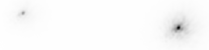We cannot tell exactly what Strehl ratio could be obtained in the vicinity of the reference star. However, the high signal-to-noise for these observations, and the high level of correlation between the stars in the close binary $\zeta$ Boötis suggest that the Strehl ratio for the reference star gives us a reasonable approximation for the Strehl ratio which would be obtained on a nearby target. The right-hand star in Figure 3.31 has a Strehl ratio only $65\%$ as high as that for the reference star. The lower Strehl ratio implies that the images of the two stars are partially decorrelated in the short exposures. This decorrelation probably results from anisoplanatism related to the separation of the binary. In order to calculate the separation from the reference star which would give a Strehl ratio of $\frac{1}{e}$ it would be necessary to know the detailed structure of the atmosphere at the time of the observations. Fitting models of the form of Equation 2.20 or similar to those of Roddier et al. (1982b) give values between

and

. Much better constraints could be put on this if wider binaries were observed - the observations in 2000 were somewhat limited by the maximum pixel rates at which the camera could operate, and hence the field of view which could be used for high frame-rate imaging. It is possible that better seeing conditions present for the runs on other targets might have also given a different (presumably larger) isoplanatic angle.

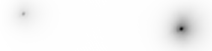
Figure 3.32 shows a shift-and-add image utilising all of the short exposures. The faint halo around the stars is more obvious in this image, but it is also much smoother in appearance. The smoothness is probably a result of the larger number of different short exposures involved, each representing a different atmospheric realisation. The Strehl ratio of the left hand star in this case is

. The Strehl ratio for the right-hand star is

, only a factor of two higher than the Strehl ratio of the long exposure seeing disk. The Strehl ratio of this star is

% as high as that for the left hand star, again suggesting significant anisoplanatism.

**Figure 3.32:** $\gamma$ Leo using left hand star as reference, all the exposures. The Strehl ratio for the left hand star is . The Strehl ratio for the right hand star is % as high as that for the left hand star.
$\begin{figure}\begin{center} \epsfig{file=not1/gleo_faint_100pc_002,width=15cm}\end{center}\end{figure}$

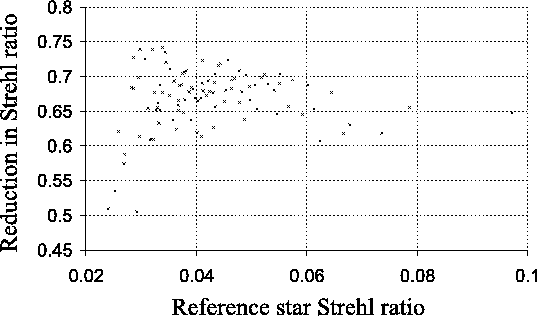
The reduction in the Strehl ratio brought about by anisoplanatism was measured using different criteria for exposure selection. The exposures of $\gamma$ Leonis were binned into one hundred equal groups each containing exposures with similar reference star Strehl ratios, as had been performed for data on $\zeta$ Boötis in Figure 3.23. The exposures in each group were shifted and co-added, resulting in a set of

images. The Strehl ratios for the reference star and the binary companion were calculated for each of these images. The high signal-to-noise ratio for these observations mean that the ratio of the binary companion Strehl to the reference star Strehl is a good measure of the reduction factor for the off-axis Strehl ratio brought about by atmospheric anisoplanatism. Figure 3.33 shows such measurements, plotted against the reference star Strehl ratio. It is clear that the fractional reduction in Strehl ratio brought about by atmospheric anisoplanatism for this data is not strongly dependent on the reference star Strehl ratio if the Strehl ratio is greater than

**Figure 3.33:** The fractional decrease in Strehl ratio for off-axis stars as measured for $\gamma$ Leonis. This plot is of the same type as Figure 3.24 but for the data on $\gamma$ Leonis. The left hand binary component was used as a reference star for measurements of the Strehl ratio and position of the brightest speckle. The exposures were then put into groups according to reference star Strehl ratio, with each group containing $1\%$ of the exposures. The fractional difference between the Strehl ratios of the two binary components is plotted against the reference star Strehl ratio in the figure.
$\begin{figure}\begin{center} \epsfig{file=not1/gleo_isoplanatics,width=12cm}\end{center}\end{figure}$

It should be noted that the fractional reduction in Strehl ratio brought about by atmospheric anisoplanatism does not provide a direct measure of the size of the isoplanatic patch. The long exposure image constructed from the same data has a Strehl ratio of

, and it will be unlikely that the Strehl ratios for short exposures would fall substantially below this value however small the isoplanatic patch. For low reference star Strehl ratios there will be a lower limit on the companion star Strehl ratio set by the finite size of the seeing disk into which most of the light from the companion star will fall (regardless of the anisoplanatism). This will tend to bias the companion star Strehl ratios obtained for low reference star Strehl ratios, and may explain why the Strehl ratios of the two stars are more similar under these conditions.

Given the lack of a model for the stratification of the atmosphere at the time of the observation, it is not possible to determine how the Strehl ratio should vary as a function of binary separation, and so we cannot say with any certainty that the isoplanatic patch is larger or smaller in the Lucky Exposures than it is in typical exposures.