Dynamic range

Figure 5.24 shows an example image generated by selecting the best $5\%$ of exposures out of $8000$ taken at $50$ $Hz$ on M13 on the night of 2003 June 29. The observations were taken through the $780$ $nm$ edge filter, with the long-wavelength cutoff determined by the sensitivity limit of the CCD (as illustrated in Figure 5.5). The $I=11.6$ star at the bottom of the image was used as a reference. The high dynamic range in this image is apparent when the image contrast is stretched one hundred fold, as demonstrated in Figure 5.25. Stars as faint as $I=18$ can be clearly detected above the noise. Stars H and W from Cohen et al. (1997) have been labelled in the image. The stars toward the top of the image have asymmetrical tails around them. The image FWHM range from $180\times110$ $mas$ for stars at the bottom of the image to $400\times220$ $mas$ for stars at the top. In order to confirm that this blurring did not result from anisoplanatism, the data analysis was repeated using star W as the reference instead of star H.

Figure 5.24: The best $5\%$ of exposures of M13 from 30 June 2003 were selected, shifted and added to produce this image with a linear greyscale. North is toward the top of the image.

Figure 5.25: Same image as for Figure 5.24 but with the greyscale contrast stretched linearly $100$ times.

Figure 5.26a shows the image of star W when star H was the reference (this is a section of the image shown in Figures 5.24 and 5.25). The asymmetry in the stellar image is very clear in this enlargement. The image of star H when star W was the reference is shown in Figure 5.26b. There is much less evidence for asymmetry in this second image (with the same angular separation of the target from the reference star) suggesting that the smearing is not a result of anisoplanatism. It appears to simply depend on the distance from the readout register of the CCD, and is consistent with poor charge transfer efficiency on the CCD (as discussed in Chapter 4.3.2). The orientation of the Figure is such that the direction of serial transfers on the CCD is downwards in the images.

Figure 5.26: The asymmetrical smearing of stellar images toward the top of Figures 5.24 and 5.25 is highlighted by the enlargement of star W shown in panel a). When star W was used as the reference, the image of star H did not show this asymmetry, as shown in panel b). This implies that the blurring is an instrumental effect and not the result of anisoplanatism.

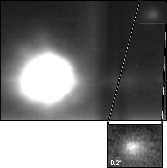
The dynamic range of Lucky Exposures is highlighted in a more quantative manner by Figure 5.27. This data on Gliese 569 was taken at a frame rate of $30$ $Hz$ on 2002 July 25 (as listed in Table 5.3). At the $810$ $nm$ observing wavelength the magnitude difference is $8$, and yet the faint companion is easily detected with little light contamination from the primary $5$ $as$ away. The data were taken through high Saharan dust extinction, and there is insufficient signal-to-noise to separate the binary components.

Figure 5.27: The best $4\%$ of exposures of the multiple star system Gliese 569. The primary star has a magnitude of $I=10$. The $I=18$ object on the right is thought to be a brown dwarf triple system (Kenworthy et al. , 2001). The images were selected from $10$ minutes of observing time at the NOT, on a night with high Saharan dust extinction at the observatory.