Returning to 2-dimensional space, we now use geometric algebra
to reveal the structure of the Argand diagram. From any vector  we can form an even multivector (a 2-dimensional
spinor):
we can form an even multivector (a 2-dimensional
spinor):

where

Using the vector  to define the real axis, there is therefore
a one-to-one correspondence between points in the
Argand diagram and vectors in two dimensions.
Complex conjugation,
to define the real axis, there is therefore
a one-to-one correspondence between points in the
Argand diagram and vectors in two dimensions.
Complex conjugation,

now appears as a natural operation of reversion for the even multivector z, and (as shown above) it is needed when rotating vectors.
We now consider the fundamental derivative operator

and observe that


Generalising this behaviour, we find that

and define an analytic function as a function  (or,
equivalently,
(or,
equivalently,  ) for which
Writing f = u + I v, this implies that

which are the Cauchy-Riemann conditions. It follows immediately that any non-negative, integer power series of z is analytic. The vector derivative is invertible so that, if

for some function s, we can find f as

Cauchy's integral formula for analytic functions is an example of this:

is simply Stokes's theorem for the plane[6]. The bivector
 is necessary to rotate the line element
  into the
direction of the outward normal.
into the
direction of the outward normal.
This definition (4.8) of
an analytic function generalises easily to higher
dimensions, where these functions are called monogenic, although
the simple link with power series disappears. Again, there are some
surprises in three dimensions. We have all learned
about the important class of harmonic functions, defined as
those functions  satisfying the scalar operator equation
Since monogenic functions satisfy
they must also be harmonic. However, this first-order equation is more
restrictive, so that not all harmonic functions are
monogenic.
In two dimensions, the solutions of equation
(4.13) are written in terms of polar coordinates
 as
as

Complex analysis tells us that there are special combinations (analytic functions) which have particular radial dependence:


In this way we can, in two dimensions, separate any given
angular component into parts regular at the origin ( ) and at
infinity (
) and at
infinity ( ). These parts are just the spinor
solutions of the first-order equation (4.14).
). These parts are just the spinor
solutions of the first-order equation (4.14).
The situation is exactly the same in three dimensions. The solutions
of  are
are

but we can find specific combinations of angular dependence which are
associated with a radial dependence of  or
or  . We
show this by example for the case l=1. Obviously, non-trivial
solutions of
. We
show this by example for the case l=1. Obviously, non-trivial
solutions of  must contain more than just a scalar part
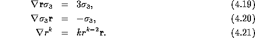
- they must be multivectors. For the position vector
must contain more than just a scalar part
- they must be multivectors. For the position vector  we find the
following relations:
we find the
following relations:
(Equation 4.20 can be derived from a more general formula given
in Section 5.) We can assemble solutions proportional to r and
 :
:
where  is the unit vector in the azimuthal direction.
Alternatively, we can generate a spherical monogenic  from any
spherical harmonic
from any
spherical harmonic  :
:

We have chosen to place the vector  to the right of
  so as
to keep
so as
to keep  within the even subalgebra of spinors. This practice is
also consistent with the conventional Pauli matrix representation
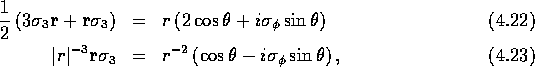
(2.20)[24]. As an example, we try this procedure
on the l=0 harmonics:
within the even subalgebra of spinors. This practice is
also consistent with the conventional Pauli matrix representation
(2.20)[24]. As an example, we try this procedure
on the l=0 harmonics:
For a selection of l=1 harmonics we obtain
Some readers may now recognise this process as similar to that
in quantum mechanics when we add the spin contribution to
the orbital angular momentum, making a total angular momentum
 . The combinations of angular dependence are the same as
in stationary solutions of the Dirac equation. In particular,
(4.25) indicates that only one monogenic arises from l=0.
That is correct - only the
. The combinations of angular dependence are the same as
in stationary solutions of the Dirac equation. In particular,
(4.25) indicates that only one monogenic arises from l=0.
That is correct - only the  state exists. Turning to
(4.26) we see that there is one state with no angular
dependence at all, and that the other has terms proportional
to
state exists. Turning to
(4.26) we see that there is one state with no angular
dependence at all, and that the other has terms proportional
to  . These can also be interpreted in terms of
  and
and  respectively.
The process by which we have generated these functions has, of course, nothing to do with quantum mechanics - another clue that many quantum-mechanical procedures are much more classical than they seem.