Limiting magnitude of reference star

In order to assess the performance with fainter reference stars, a field in the globular cluster M13 was observed with stars having a wide range of different magnitudes on 2001 July 26. The observations are listed as M13 field 2 in Table 5.2. A Lucky Exposures image of the field using $1\%$ of the $6000$ exposures with this telescope pointing is shown in Figure 5.16a. The $I=12.7$ star labelled Z in the image was used as the reference for image selection and re-centring in this case. The frame rate used for these observations was $18$ $Hz$, giving a total integration time on the sky of $330$ $s$. Star A from Cohen et al. (1997) is labelled in the figure. This star was saturated in the best short exposures, and has hence been omitted from further analyses. The stellar image FWHM of $\sim100$ $mas$ are very competitive with other imaging techniques. The image shows faint asymmetrical horizontal tails around the fainter stars, which may be evidence of poor charge transfer efficiency (vertical tails are also visible in the cross-sections of Figure 5.16b). The electrical heating was not connected at the time these runs were taken, so it is plausible that the charge transfer efficiency might have been poorer here than during other runs on the same night. Despite this effect, the stellar cores throughout the image are extremely compact.

Figure 5.16: The best $1\%$ of exposures of M13 were selected and re-centred to produce the near diffraction-limited image shown in a). Star A from Cohen et al. (1997) has been labelled. The $I=12.7$ star Z was the reference star used for image selection. Panel b) shows cross-sections through stars X and Y along the lines indicated in panel a).

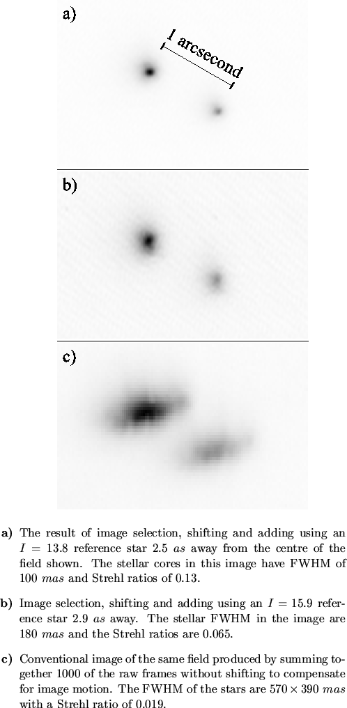
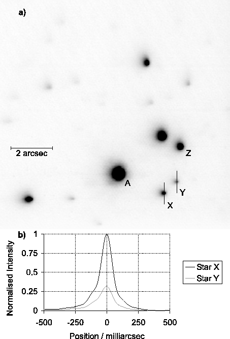
The analysis of this data was repeated using a range of different stars in the field as the reference for exposure selection and re-centring. The Lucky Exposures method was found to work very successfully with relatively faint reference stars. First the $I=13.8$ star labelled X in Figure 5.16 was used as a reference for selecting the best $1\%$ of exposures and re-centring them. A section of the resulting image (the region around the star labelled Z in Figure 5.16) is shown in Figure 5.17a. Note that neither of the two stars visible in this figure was used as the reference in this case (star X was used) and yet the stellar cores are extremely sharp. The Strehl ratio for the stars in this image was measured as $0.13$. Figure 5.17b shows a similar image generated using an $I=15.9$ reference star. The Strehl ratio of $0.065$ still represents a substantial improvement over the Strehl ratio of $0.019$ for the averaged (long exposure) image shown in Figure 5.17c. The image FWHM of $180$ $mas$ for Figure 5.17b would be extremely valuable for many astrophysical programs, and represents an enormous improvement over the $570\times390$ $mas$ for the long exposure image. The asymmetry in the long exposure image might be the result of telescope tracking errors, as M13 was close to the zenith. The position of the brightest speckle in the image of a reference star shows jumps in the horizontal direction, as can be seen in Figure 5.18.

Figure 5.17: a)--c) Image resolution for a field in M13 with different reference stars.

Figure 5.18: The position of the brightest speckle measured in the image of star $Z$ in our exposures (see Figure 5.16) as a function of time. The upper plot shows the vertical offset from the mean position for the brightest speckle, and the lower plot shows the horizontal offset.

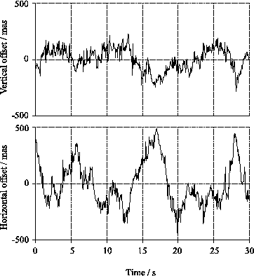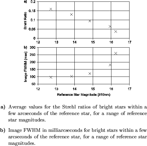
Figure 5.19 shows plots of the variation in the Strehl ratio and FWHM of nearby stars when a range of different stars are used as the reference for image selection and for the shifting and adding process. $1\%$ of the exposures were selected in the analyses used to generate these plots, and the Strehl ratios and FWHM were calculated using nearby stars in order to minimise the effects of anisoplanatism. Figure 5.19a shows the decline in Strehl ratio with increasingly faint reference star magnitude. The Strehl ratio of the Lucky Exposures image remains substantially higher than the seeing-limited value of $0.019$ even for reference stars as faint as $I=16$. Figure 5.19b shows the image FWHM obtained using the same reference stars. An image FWHM of $100$ $mas$ can be achieved using reference stars as faint as $I=14$, and there is a substantial improvement over the FWHM for the seeing-limited image of $570\times390$ $mas$ even for $I=15.9$ reference stars.

Figure 5.19: a), b) Image resolution for a range of different reference stars in M13.

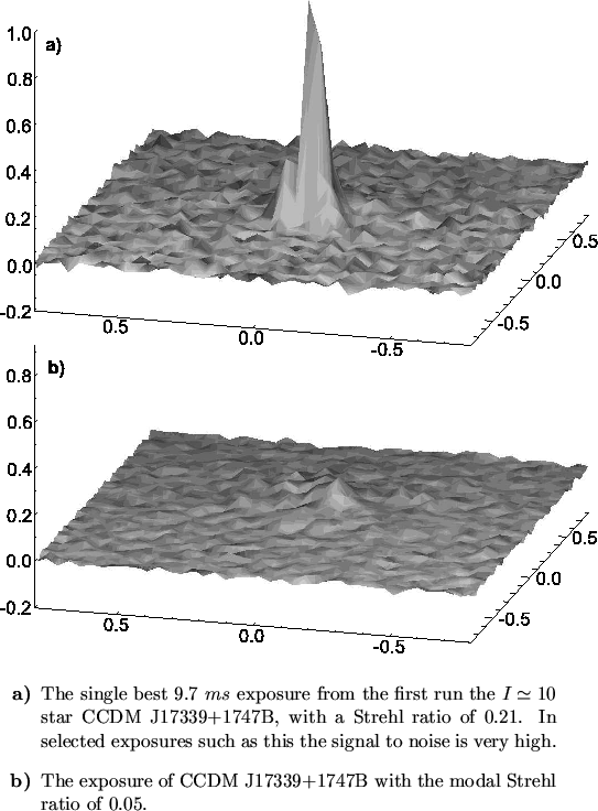
The faint limiting magnitude for the Lucky Exposures method stems partly from the high signal-to-noise ratio for measurements of the brightest speckle in those exposures having the highest Strehl ratios. This is highlighted in Figure 5.20, which shows surface plots of two frames taken from a run on the $I=10$ star CCDM J17339+1747B on 2001 July 26 (listed in Table 5.2). Figure 5.20a shows an exposure with a high Strehl ratio ($0.21$). The location and Strehl ratio of the brightest speckle in this image can be measured with a high signal-to-noise ratio. Good results would be obtained if exposures such as this were re-centred based on the location of the brightest speckle. In contrast, Figure 5.20b shows a typical exposure with poorer Strehl ratio. The brightest speckle has a peak flux which is barely above the noise level, and the errors in determining the location of the brightest speckle will be substantially higher in this case. If a large fraction of the exposures are selected and re-centred, these errors would lead to poorer image quality for other objects in the field around the reference star. Conversely, if only those exposures with high Strehl ratios are used, we would expect the re-centring errors to be smaller. Combined with the higher intrinsic Strehl ratios in the selected exposures, these should lead to much higher image resolution for objects in the field.

Figure 5.20: a), b) Surface plots of intensity in two example exposures taken from a run on the faint star CCDM J17339+1747B. The exposures had a duration of $9.7$ $ms$.

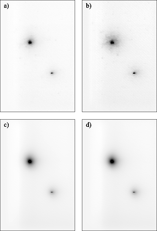
The Lucky Exposures image quality obtained from the run on CCDM J17339+1747AB is summarised in Figure 5.21. The lower right $I=10$ star was the one shown in Figure 5.20, and this star was used as the reference for exposure selection and re-centring. Figure 5.21a shows the image obtained by selecting and re-centring the best $1\%$ of exposures based on the brightest pixel in the filtered exposures in the usual way. Figure 5.21b shows the result obtained if the brightest pixel in the raw short exposures is used without Fourier filtering using the function shown in Figure 5.6 for calculations of the Strehl ratio and position of the brightest speckle. The halo around the bright star is clearly less compact in this image. Figures 5.21c and 5.21d show images generated in the same way but using all of the exposures. The re-centring process was based on the position of the brightest pixel in the raw exposures for the fainter star at the lower right for Figures 5.21d. Despite the relatively low signal-to-noise ratio apparent in Figure 5.20, the re-centring process has reduced the image FWHM to $120$ $mas$ from $0.5$ $as$ achieved without re-centring. Good image quality is obtained at this signal-to-noise even without filtering out the noise.

Figure 5.21: Results of exposure selection on CCDM J17339+1747AB. For a), the best $1\%$ of exposures were selected using the standard approach. b) shows the result without the use of Fourier filtering to suppress noise in the exposure selection step. c) and d) are the same as a) and b) but using all of the exposures.

Using the flux calibration for an A0 V star in Cox (2000) and the predicted throughput of the telescope, instrument, filter and CCD quantum efficiency shown Figure 5.5 I calculated the number of detected photons expected from a $I=15.9$ reference star in a single $55$ $ms$ exposure. The total transmission under curve B corresponds to an equivalent bandpass of $23$ $nm$ with $100\%$ transmission. Using a value of $6.1\times 10^{-15}$ $W$ $m^{-2}$ $nm^{-1}$ for the flux from an $I=15.9$ at $810$ $nm$ wavelength this would imply a rate of $1.2\times 10^{5}$ detected photons per second. In a $55$ $ms$ exposure we would thus expect about $5900$ photons. If the Strehl ratio in a good exposure is $0.2$, $20\%$ of this flux will fall in one bright speckle (corresponding to about $1200$ photons). Taking the simplified model for the signal-to-noise ratio with L3Vision CCDs described by Equation 4.20, we expect a signal-to-noise ratio of about $24$ on such a speckle.