Temperature Analysis

Three-Year Wilkinson Microwave Anisotropy Probe (WMAP) Observations: Temperature Analysis, G. Hinshaw, et al., 2007, ApJS, 170, 288, reprint / preprint (1.3MB) / bundled figures (18.5MB) / individual figures / ADS / astro-ph

WMAP Three-year Paper Figures, Hinshaw et al.
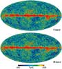
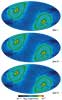
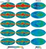
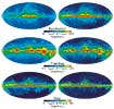
Individual figures are provided for use in talks. Proper display of PNG transparency in PowerPoint requires saving files to your computer before Inserting them. Please acknowledge the WMAP Science Team when using these images. Image Credit: NASA / WMAPScience Team
	Fig. 1a Full-sky maps in Galactic coordinates smoothed with a 0.2°; Gaussian beam, shown in Mollweide projection. top K-band (23 GHz), middle Ka-band (33 GHz), bottom Q-band (41 GHz).	PNG (775 kb - 512x841 pixels) PNG (3.5 mb - 1024x1682 pixels) EPS (5.6 mb)
	Fig. 1b Full-sky maps in Galactic coordinates smoothed with a 0.2° Gaussian beam, shown in Mollweide projection. top V-band (61 GHz), bottom W-band (94 GHz).	PNG (608 kb - 512x572 pixels) PNG (3.0 mb - 1024x1144 pixels) EPS (4.9 mb)
	Fig. 2 The number of independent W-band observations per pixel in Galactic coordinates, top: year-1, middle: year-2, and bottom: year-3. The number of observations is greatest near the ecliptic poles and in rings approximately 141° from each pole.	PNG (552 kb - 552x885 pixels) PNG (2.8 mb - 1104x1769 pixels) EPS (1.5 mb)
	Fig. 3 Comparison of the three-year maps with the previously released one-year maps. The data are smoothed to 1° resolution and are shown in Galactic coordinates. The frequency bands K through W are shown top to bottom.	PNG (468 kb - 512x548 pixels) PNG (2.0 mb - 1024x1096 pixels) EPS (1.2 mb)
	Fig. 4 Results from the MEM foreground degeneracy analysis. (a) The spectrum of total foreground emission (diamonds) compared to the sum of the MEM components (lines connecting the diamonds), averaged over the full sky.	PNG (22 kb - 495x512 pixels) PNG (58 kb - 989x1024 pixels) EPS (223 kb)
	Fig. 5 Galactic signal component maps from the Maximum Entropy Method (MEM) analysis (§4.5). top-bottom: synchrotron, free-free, and dust emission with logarithmic temperature scales, as indicated.	PNG (413 kb - 527x552 pixels) PNG (1.9 mb - 1053x1104 pixels) EPS (931 kb)
	Fig. 6 The mean Galaxy spectrum from 408 MHz to 94 GHz, based on data from Haslam, Tenerife and WMAP. Each point is the mean signal in the Galactic latitude range 20°< |b| < 50° with the mean at the Galactic poles subtracted.	PNG (11 kb - 386x512 pixels) PNG (24 kb - 771x1024 pixels) EPS (102 kb)
	Fig. 7 An overview of the microwave sky. The yellow, salmon, and red shaded regions indicate the Kp0, Kp2, and Kp8 diffuse emission masks where the Galactic foreground signal is especially strong.	PNG (42 kb - 383x750 pixels) PNG (112 kb - 765x1500 pixels) EPS (594 kb)
	Fig. 8 top: Full-sky map color-coded to show the 12 regions that were used to generate the three-year ILC map (see §5.2). bottom: The mean ILC residual map from 100 Monte Carlo simulations of CMB signal, Galactic foreground signal and instrument noise.	PNG (316 kb - 512x577 pixels) PNG (1.3 mb - 1024x1153 pixels) EPS (543 kb)
	Fig. 9 top: The first-year ILC map reproduced from Bennett et al. (2003c). middle: The three-year ILC map produced following the steps outlined in §5.2. bottom: The difference between the two (1-yr - 3-yr).	PNG (775 kb - 512x890 pixels) PNG (3.2 mb - 1024x1779 pixels) EPS (968 kb)
	Fig. 10 Galactic foreground removal with spatial templates. All maps in this figure are three-year maps that have had the ILC estimate of the CMB signal subtracted off to highlight the foreground emission.	PNG (355 kb - 343x512 pixels) PNG (1.2 mb - 686x1024 pixels) EPS (1.4 mb)
	Fig. 11 Measurement of the source number count distribution dN/dS.	PNG (19 kb - 383x512 pixels) PNG (37 kb - 765x1024 pixels) EPS (123 kb)
	Fig. 12 The predicted Cl uncertainty (inverse Fisher matrix) at low l, in μK4. The red curves show the result when pixel-pixel noise correlations are ignored. The smooth rise at low l reflects our approximate representation of 1/f noise in the noise bias model.	PNG (17 kb - 358x512 pixels) PNG (34 kb - 715x1024 pixels) EPS (200 kb)
	Fig. 13 (top) Q-, V-, & W-band cross-power spectra before foreground subtraction, evaluated outside the Kp2 sky cut, relative to the final combined spectrum. (bottom) Same cross-power spectra after subtracting a template-based diffuse foreground model (§5.3) and the best-fit residual point source contamination (§7.2).	PNG (12 kb - 423x512 pixels) PNG (26 kb - 846x1024 pixels) EPS (120 kb)
	Fig. 14 Maps of power spectrum modes l = 2 - 8 computed from full-sky fits to the ILC map, shown at top left. Many authors note peculiar patterns in the phase of these modes, and many claim that the behavior is inconsistent with Gaussian random-phase fluctuations, as predicted by inflation.	PNG (362 kb - 506x512 pixels) PNG (1.2 mb - 1012x1024 pixels) EPS (642 kb)
	Fig. 15 The posterior likelihood of l(l + 1)Cl/2π given the WMAP data, for l=2-10. The curves are computed using data from the ILC map evaluated outside the Kp2 sky cut. The vertical blue lines show the values inferred using the pseudo-Cl estimate.	PNG (19 kb - 503x512 pixels) PNG (44 kb - 1005x1024 pixels) EPS (186 kb)
	Fig. 16 The binned three-year angular power spectrum (in black) from l=2-1000, where it provides a cosmic variance limited measurement of the first acoustic peak, a robust measurement of the second peak, and clear evidence for rise to the third peak.	PNG (11 kb - 367x512 pixels) PNG (26 kb - 734x1024 pixels) EPS (157 kb)
	Fig. 17 X² vs. l for the full power spectrum relative to the best-fit ΛCDM model, fit to WMAP data only. The X² per l has been averaged in l-bands of width Δl = 15. The dark to light grey shading indicates the 1, 2, and 3σ confidence intervals for this distribution.	PNG (9 kb - 352x512 pixels) PNG (19 kb - 704x1024 pixels) EPS (120 kb)
	Fig. 18 The WMAP three-year power spectrum (in black) compared to other recent measurements of the CMB angular power spectrum, including Boomerang (Jones et al. 2005), Acbar (Kuo et al. 2004), CBI (Readhead et al. 2004), and VSA (Dickinson et al. 2004).	PNG (10 kb - 366x512 pixels) PNG (24 kb - 732x1024 pixels) EPS (164 kb)
	Fig. 19 Comparison of the three-year angular power spectrum with the first-year result. (top) The three-year combined spectrum, in black, is shown with the first-year spectrum, as published, in red. The best-fit three-year ΛCDM model is shown in grey for comparison.	PNG (9 kb - 250x512 pixels) PNG (22 kb - 500x1024 pixels) EPS (184 kb)
	Fig. 20 The unbinned three-year angular power spectrum (in black) from l=2-400, where it provides a cosmic variance limited measurement of the first acoustic peak. The first-year spectrum is shown in green for comparison.	PNG (14 kb - 387x512 pixels) PNG (39 kb - 774x1024 pixels) EPS (146 kb)
	Fig. 21 Full-sky ILC map in ecliptic coordinates smoothed to 1° resolution, shown in Lambert Azimuthal Equal Area projection.	PNG (261 kb - 305x512 pixels) PNG (1.0 mb - 609x1024 pixels) EPS (635 kb)
	Fig. 22 Angular power spectra ClTT & ClTE from the three-year WMAP data. top: The TT data are as shown in Figure 16. The TE data are shown in units of l(l+1)Cl/2π, on the same scale as the TT signal for comparison. bottom: The TE data, in units of (l + 1)Cl/2π.	PNG (11 kb - 413x512 pixels) PNG (24 kb - 825x1024 pixels) EPS (181 kb)
	Fig. 23 An estimate of the multiplicative error introduced in the angular power spectrum, Cl, due to the effects of beam asymmetry. See §7.1.1 and Appendix B for details on how this estimate was obtained.	PNG (10 kb - 436x512 pixels) PNG (23 kb - 872x1024 pixels) EPS (145 kb)